Scoring and Ranking
Scoring and Ranking. 198:541 Spring 2007. Scoring. Thus far, our queries have all been Boolean Docs either match or not Good for expert users with precise understanding of their needs and the corpus Applications can consume 1000’s of results

Scoring and Ranking
E N D
Presentation Transcript
Scoring and Ranking 198:541 Spring 2007
Scoring • Thus far, our queries have all been Boolean • Docs either match or not • Good for expert users with precise understanding of their needs and the corpus • Applications can consume 1000’s of results • Not good for (the majority of) users with poor Boolean formulation of their needs • Most users don’t want to wade through 1000’s of results – cf. use of web search engines
Scoring • We wish to return in order the documents most likely to be useful to the searcher • How can we rank order the docs in the corpus with respect to a query? • Assign a score – say in [0,1] • for each doc on each query • Begin with a perfect world – no spammers • Nobody stuffing keywords into a doc to make it match queries • More on “adversarial IR” under web search
Linear zone combinations • First generation of scoring methods: use a linear combination of Booleans: • E.g., Score = 0.6*<sorting in Title> + 0.3*<sorting in Abstract> + 0.05*<sorting in Body> + 0.05*<sorting in Boldface> • Each expression such as <sorting in Title> takes on a value in {0,1}. • Then the overall score is in [0,1]. For this example the scores can only take on a finite set of values – what are they?
Linear zone combinations • In fact, the expressions between <> on the last slide could be any Boolean query • Who generates the Score expression (with weights such as 0.6 etc.)? • In uncommon cases – the user, in the UI • Most commonly, a query parser that takes the user’s Boolean query and runs it on the indexes for each zone
General idea • We are given a weight vector whose components sum up to 1. • There is a weight for each zone/field. • Given a Boolean query, we assign a score to each doc by adding up the weighted contributions of the zones/fields. • Typically – users want to see the K highest-scoring docs.
Where do these weights come from? • Machine learned relevance • Given • A test corpus • A suite of test queries • A set of relevance judgments • Learn a set of weights such that relevance judgments matched • Can be formulated as ordinal regression
Full text queries • We just scored the Boolean query bill OR rights • Most users more likely to type billrights or bill of rights • How do we interpret these full text queries? • No Boolean connectives • Of several query terms some may be missing in a doc • Only some query terms may occur in the title, etc.
Full text queries • To use document combinations for free text queries, we need • A way of assigning a score to a pair <free text query, document> • Zero query terms in the document should mean a zero score • More query terms in the document should mean a higher score • Scores don’t have to be Boolean • Will look at some alternatives now
Incidence matrices • Recall: Document (or a zone in it) is binary vector X in {0,1}v • Query is a vector • Score: Overlap measure:
Example • On the query ides of march, Shakespeare’s Julius Caesar has a score of 3 • All other Shakespeare plays have a score of 2 (because they contain march) or 1 • Thus in a rank order, Julius Caesar would come out tops
Overlap matching • What’s wrong with the overlap measure? • It doesn’t consider: • Term frequency in document • Term scarcity in collection (document mention frequency) • of is more common than ides or march • Length of documents • (And queries: score not normalized)
Scoring: density-based • Thus far: position and overlap of terms in a doc – title, author etc. • Obvious next: idea if a document talks about a topic more, then it is a better match • This applies even when we only have a single query term. • Document relevant if it has a lot of the terms • This leads to the idea of term weighting.
Term-document count matrices • Consider the number of occurrences of a term in a document: • Bag of words model • Document is a vector in ℕv: a column below
Bag of words view of a doc • Thus the doc • John is quicker than Mary. is indistinguishable from the doc • Mary is quicker than John. Which of the indexes discussed so far distinguish these two docs?
Counts vs. frequencies • Consider again the ides of march query. • Julius Caesar has 5 occurrences of ides • No other play has ides • march occurs in over a dozen • All the plays contain of • By this scoring measure, the top-scoring play is likely to be the one with the most ofs
Digression: terminology • WARNING: In a lot of IR literature, “frequency” is used to mean “count” • Thus term frequency in IR literature is used to mean number of occurrences in a doc • Not divided by document length (which would actually make it a frequency) • We will conform to this misnomer • In saying term frequency we mean the number of occurrences of a term in a document.
Term frequency tf • Long docs are favored because they’re more likely to contain query terms • Can fix this to some extent by normalizing for document length • But is raw tf the right measure?
Weighting term frequency: tf • What is the relative importance of • 0 vs. 1 occurrence of a term in a doc • 1 vs. 2 occurrences • 2 vs. 3 occurrences … • Unclear: while it seems that more is better, a lot isn’t proportionally better than a few • Can just use raw tf • Another option commonly used in practice:
Score computation • Score for a query q = sum over terms t in q: • [Note: 0 if no query terms in document] • This score can be zone-combined • Can use wf instead of tf in the above • Still doesn’t consider term scarcity in collection (ides is rarer than of)
Weighting should depend on the term overall • Which of these tells you more about a doc? • 10 occurrences of hernia? • 10 occurrences of the? • Would like to attenuate the weight of a common term • But what is “common”? • Suggest looking at collection frequency (cf ) • The total number of occurrences of the term in the entire collection of documents
Document frequency • But document frequency (df ) may be better: • df = number of docs in the corpus containing the term Word cfdf ferrari 10422 17 insurance 10440 3997 • Document/collection frequency weighting is only possible in known (static) collection. • So how do we make use of df ?
tf x idf term weights • tf x idf measure combines: • term frequency (tf ) • or wf, some measure of term density in a doc • inverse document frequency (idf ) • measure of informativeness of a term: its rarity across the whole corpus • could just be raw count of number of documents the term occurs in (idfi = 1/dfi) • but by far the most commonly used version is: • See Kishore Papineni, NAACL 2, 2002 for theoretical justification
Summary: tf x idf (or tf.idf) • Assign a tf.idf weight to each term i in each document d • Increases with the number of occurrences within a doc • Increases with the rarity of the term across the whole corpus What is the wt of a term that occurs in all of the docs?
Inverse Document Frequency • IDF provides high values for rare words and low values for common words For a collection of 10000 documents
Real-valued term-document matrices • Function (scaling) of count of a word in a document: • Bag of words model • Each is a vector in ℝv • Here log-scaled tf.idf Note can be >1!
Documents as vectors • Each doc j can now be viewed as a vector of wfidf values, one component for each term • So we have a vector space • terms are axes • docs live in this space • even with stemming, may have 20,000+ dimensions • (The corpus of documents gives us a matrix, which we could also view as a vector space in which words live – transposable data)
Why turn docs into vectors? • First application: Query-by-example • Given a doc d, find others “like” it. • Now that d is a vector, find vectors (docs) “near” it.
Intuition t3 d2 d3 d1 θ φ t1 d5 t2 d4 Postulate: Documents that are “close together” in the vector space talk about the same things.
Desiderata for proximity • If d1 is near d2, then d2 is near d1. • If d1 near d2, and d2 near d3, then d1 is not far from d3. • No doc is closer to d than d itself.
First cut • Idea: Distance between d1 and d2 is the length of the vector |d1 – d2|. • Euclidean distance • Why is this not a great idea? • We still haven’t dealt with the issue of length normalization • Short documents would be more similar to each other by virtue of length, not topic • However, we can implicitly normalize by looking at angles instead
t 3 d 2 d 1 θ t 1 t 2 Cosine similarity • Distance between vectors d1 and d2captured by the cosine of the angle x between them. • Note – this is similarity, not distance • No triangle inequality for similarity.
Cosine similarity • A vector can be normalized (given a length of 1) by dividing each of its components by its length – here we use the L2 norm • This maps vectors onto the unit sphere: • Then, • Longer documents don’t get more weight
Cosine similarity • Cosine of angle between two vectors • The denominator involves the lengths of the vectors. Normalization
Normalized vectors • For normalized vectors, the cosine is simply the dot product:
Example • Docs: Austen's Sense and Sensibility, Pride and Prejudice; Bronte's Wuthering Heights. tf weights • cos(SAS, PAP) = .996 x .993 + .087 x .120 + .017 x 0.0 = 0.999 • cos(SAS, WH) = .996 x .847 + .087 x .466 + .017 x .254 = 0.889
Queries in the vector space model Central idea: the query as a vector: • We regard the query as short document • We return the documents ranked by the closeness of their vectors to the query, also represented as a vector. • Note that dq is very sparse!
Summary: What’s the point of using vector spaces? • A well-formed algebraic space for retrieval • Key: A user’s query can be viewed as a (very) short document. • Query becomes a vector in the same space as the docs. • Can measure each doc’s proximity to it. • Natural measure of scores/ranking – no longer Boolean. • Queries are expressed as bags of words • Other similarity measures: see http://www.lans.ece.utexas.edu/~strehl/diss/node52.html for a survey
Interaction: vectors and phrases • Scoring phrases doesn’t fit naturally into the vector space world: • “tangerine trees” “marmalade skies” • Positional indexes don’t calculate or store tf.idf information for “tangerine trees” • Biword indexes treat certain phrases as terms • For these, we can pre-compute tf.idf. • Theoretical problem of correlated dimensions • Problem: we cannot expect end-user formulating queries to know what phrases are indexed • We can use a positional index to boost or ensure phrase occurrence
Vectors and Boolean queries • Vectors and Boolean queries really don’t work together very well • In the space of terms, vector proximity selects by spheres: e.g., all docs having cosine similarity 0.5 to the query • Boolean queries on the other hand, select by (hyper-)rectangles and their unions/intersections • Round peg - square hole
1,2 7,3 83,1 87,2 … 1,1 5,1 13,1 17,1 … 7,1 8,2 40,1 97,3 … aargh 10 abacus 8 acacia 35 Encoding document frequencies • Add tft,d to postings lists • Now almost always as frequency – scale at runtime • Overall, requires little additional space
Computing the k largest cosines: selection vs. sorting • Typically we want to retrieve the top k docs (in the cosine ranking for the query) • not to totally order all docs in the corpus • Can we pick off docs with k highest cosines?
Limiting the accumulators:Best m candidates • Preprocess: Pre-compute, for each term, its m nearest docs. • (Treat each term as a 1-term query.) • lots of preprocessing. • Result: “preferred list” for each term. • Search: • For a t-term query, take the union of their t preferred lists – call this set S, where|S| mt. • Compute cosines from the query to only the docs in S, and choose the top k. Need to pick m>k to work well empirically.
Measures for a search engine • How fast does it index • Number of documents/hour • (Average document size) • How fast does it search • Latency as a function of index size • Expressiveness of query language • Ability to express complex information needs • Speed on complex queries
Measures for a search engine • All of the preceding criteria are measurable: we can quantify speed/size; we can make expressiveness precise • The key measure: user happiness • What is this? • Speed of response/size of index are factors • But blindingly fast, useless answers won’t make a user happy • Need a way of quantifying user happiness
Measuring user happiness • Issue: who is the user we are trying to make happy? • Depends on the setting • Web engine: user finds what they want and return to the engine • Can measure rate of return users • eCommerce site: user finds what they want and make a purchase • Is it the end-user, or the eCommerce site, whose happiness we measure? • Measure time to purchase, or fraction of searchers who become buyers?
Measuring user happiness • Enterprise (company/govt/academic): Care about “user productivity” • How much time do my users save when looking for information? • Many other criteria having to do with breadth of access, secure access, etc.