Download
1 / 43
430 likes | 466 Vues
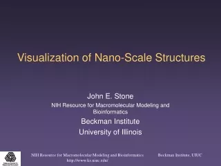
Visualization of Nano-Scale Structures. John E. Stone NIH Resource for Macromolecular Modeling and Bioinformatics Beckman Institute University of Illinois. VMD. VMD – “Visual Molecular Dynamics” Visualization of molecular dynamics simulations, sequence data, volumetric data

E N D
Visualization of Nano-Scale Structures John E. Stone NIH Resource for Macromolecular Modeling and Bioinformatics Beckman Institute University of Illinois
VMD • VMD – “Visual Molecular Dynamics” • Visualization of molecular dynamics simulations, sequence data, volumetric data • User extensible with scripting and plugins • http://www.ks.uiuc.edu/Research/vmd/
Overview • Will be showing a lot of VMD images, feel free to ask questions • General visualization concepts and methods • Specific visualization examples for molecular dynamics trajectories, CryoEM maps, etc. • Graphics technology driving molecular visualization capabilities and performance • Challenges encountered exploiting these technologies for our purposes • Where things are headed…
What is Visualization? Visualize: "to form a mental vision, image, or picture of (something not visible or present to sight, or of an abstraction); to make visible to the mind or imagination"[The Oxford English Dictionary]
Goals of Visualization • Exploring data, making the invisible visible • Gaining insight and understanding, interpret the meaning of the data • Interactivity • Communicating with others
Attributes of the Data We’re Interested in Visualizing • Multiple types of data • Atomic structures • Sequence Data • Volumetric data • Many attributes per-atom • Millions of atoms, voxels • Time varying (simulation trajectories) • Multiple structures
Visualizing Data with Shape • Direct rendering of geometry from physical data (e.g. atomic structures) • Indirect rendering of data, feature extraction (e.g. density isosurfaces) • Reduced detail representations of data (e.g. ribbons, cartoon) • Use size for emphasis
Schematic Representations • Extract and render pores, cavities, indentations • Simplified representations of large structures
Visualizing Data with Texture and Color • Direct mapping of properties/values to colors (e.g. color by electrostatic potential) • Indirect mapping via feature extraction (e.g. color by secondary structure) • Use saturated colors to draw attention • Use faded colors and transparency to de-emphasize • Use depth cueing/fog to de-emphasize background environment
Visualizing Data Topologically • Data relationships indicated by grouping (e.g. phylogenetic trees) • Abstract or schematic representation (e.g. Ramachandran plot)
Bringing it all together… • Aligned sequences and structures, phylogeny • Simultaneous use of shape, color, topology, and interactivity • Multiple simultaneous representations • Multiple data display modalities • Selections in one modality can be used to highlight or select in others
What else can we do? • Enhance visual perception of shape • Motion, interactive rotation • Stereoscopic display • High quality surface shading and lighting • Enhance tactile perception of shape • Print 3-D solid models • Interactive exploration using haptic feedback
VMD Representation Examples • Draw atomic structure, protein backbone, secondary structure, solvent-accessible surface, window-averaged trajectory positions, isosurfaces of volumetric data, much more… • Color by per-atom or per-residue info, position, time, electrostatic potential, density, user-defined properties, etc… Ribosome, J. Frank GroEL /w Situs 4HRV, 400K atoms
Multiple Representations, Cut-away Views • Multiple reps are often used concurrently • Show selected regions in full atomic detail • Simplified cartoon-like or schematic form • Clipping planes can slice away structure obscuring interesting features
GroEL: Docked Map and Structure • SITUS + VMD since 1999 • SITUS: • Dock map+structure • Synthesize map from PDB • Calculate difference between EM map and PDB • VMD: • Load SITUS maps or meshes • Display isosurfaces • Display map/structure alignment error as isosurfaces • Texture reps by density or map/structure alignment error
GroEL: Display of Difference, Error Ribbons textured by difference map …with difference isosurfaces
GroEL: Select Atoms by Map Values • Superimpose the difference map isosurface with VDW rep of atoms in difference areas • Atoms can be selected by map values: • Nearest voxel • Interpolated voxel value • Selections can be used for purposes other than visualization, scripting, etc.
RDV: Fast, Coarse Map Display • Shaded points can be rendered very efficiently • Normals are retrieved from a volume gradient map that VMD generates when maps are loaded • Effective for dense surfaces • Even a 3 yr. old laptop can interactively rotate a shaded points isosurface of the 230x230x140 RDV map
Trajectory Animation • Motion aids perception of shape, understanding of dynamic processes • Animate entire model, or just the parts where motion provides insight • Window-average positions on-the-fly to focus on significant motions • Selected atoms updated on-the-fly (distance constraints, etc)
Visualization of Large All Atom Molecular Dynamics Simulations (1) • All-atom models of proteins, membranes, DNA, in water solution • 100K to 2M atoms • 512 CPU jobs run on remote supercomputers for weeks at a time for a 10ns simulation • Visualization and analysis require workstations with 4-32 GB of RAM, 1-4 CPUs, high-end graphics accelerators
Visualization of Large All Atom Molecular Dynamics Simulations (2) • Multiple representations show areas in appropriate detail • Large models: 1,00,000 atoms and up • Long trajectories: thousands of timesteps • A 10 ns simulation of 100K atoms produces a 12GB trajectory • Multi-gigabyte data sets break 32-bit addressing barriers Purple Membrane 150,000 Atoms F1 ATPase 327,000 Atoms
Visualization of Large All Atom Molecular Dynamics Simulations (3) Satellite Tobacco Mosaic Virus 932,508 atoms Coarse Representation
Visualizing Coarse-Grain Simulations Satellite Tobacco Mosaic Virus, CG Model • Visualization techniques can be used for both all-atom and CG models • Groups of atoms replaced with “beads”, surface reps, or other geometry • Display 1/20th the data • No standard file formats for CG simulation trajectories yet, done with scripting currently
User Interface Issues • Ease of use is important • Graphical picking and text-based selection languages need higher level selection keywords to work well with huge complexes • Viewing huge structures involves more clutter, even with coarse reps, software must do more to help you see what you want to see automatically • Software needs to know what’s “important” at a higher level, much of this information must come from the structure/map files themselves
Comparison of Molecular Visualization with Other Graphics Intensive Applications Texture/Shading Complexity • Geometric complexity limits molecular visualization performance • All atoms move every simulation timestep, thwarts many simplification techniques • Commodity graphics hardware is tuned for requirements of games • Solution: Use sophisticated shading instead of geometry where possible PIXAR, ILM Movie Studios Games Flight Simulation Biomolecular Visualization HW Trend CAD Geometric Complexity
Timeline: Graphics Hardware Used for Molecular Visualization 60’s and 70’s: Mainframe-based vector graphics on Tektronix terminals Evans & Sutherland graphics machines 80’s: Transition to raster graphics on Unix workstations, Mac, PC Space-filling molecular representations Stereoscopic rendering 90’s - 2002: 3rd-generation raster graphics systems Depth-cueing Texture mapping: coloring by potential, density, etc Full-scene antialiasing
Programmable Graphics Hardware Groundbreaking research systems: AT&T Pixel Machine (1989): 82 x DSP32 processors UNC PixelFlow (1992-98): 64 x (PA-8000 + 8,192 bit-serial SIMD) SGI RealityEngine (1990s): Up to 12 i860-XP processors perform vertex operations (ucode), fixed-func fragment hardware Most graphics boards now incorporate programmable processors at some level UNC PixelFlow Rack Reality Engine Vertex Processors
GPUs Already Outperformed CPUs for Raw Arithmetic In 2004.The Performance Gap Continues to Widen..… Floating point multiply-add performance (Data courtesey Ian Buck) NVIDIA NV30, 35, 40 ATI R300, 360, 420 GFLOPS Intel Pentium 4 July 01 Jan 02 July 02 Jan 03 July 03 Jan 04
Programmable Shading: Computational Power Enables New Visualization and Analysis Techniques Multiply Add Performance NVIDIA GeForceFX 7800 3.0 GHz dual-core Pentium4 Courtesy Ian Buck, John Owens
Early Experiments with Programmable Graphics Hardware in VMD • Sun XVR-1000/4000 (2002) • 4xMAJC-5200 CPUs • 1GB Texture RAM • 32MB ucode RAM • 1 Teraflop Antialiasing Filter Pipeline • Custom ucode and OpenGL extension for rendering spheres • Draw only half-spheres, with solid side facing the viewer • 1-sided lighting • Host CPU only sends arrays of radii, positions, colors • fast DMA engines copy arrays from system memory to GPU • Overall performance twice as fast, host CPU load significantly decreased
Benefits of Programmable Shading (1) Fixed-Function OpenGL • Potential for superior image quality with better shading algorithms • Direct rendering of: • Quadric surfaces • Density map data, solvent surfaces • Offload work from host CPU to GPU Programmable Shading: - same tessellation -better shading
Benefits of Programmable Shading (2) Myoglobin cavity “openness” (time averaged spatial occupancy) Single-level OpenGL screen-door transparency obscures internal surfaces Programmable shading shows transparent nested probability density surfaces with similar performance
Rendering Non-polygonal Data with Present-day Programmable Shading • Algorithms mapped to vertex/fragment shading model available in current hardware • Render by drawing bounding box or a viewer-directed quad containing shape/data • Vertex shader sets up • Fragment shader performs all the work Fragment shader is evaluated for all pixels rasterized by bounding box. Contained object could be anything one can render in a point-sampled manner (e.g. scanline rendering or ray tracing of voxels, triangles, spheres, cylinders, tori, general quadric surfaces, etc…)
Ray Traced Sphere Rendering with Programmable Shading Fixed-Function OpenGL: 512 triangles per sphere • Fixed-function OpenGL requires curved surfaces to be tessellated with triangles, lines, or points • Fine tessellation required for good results with Gouraud shading; performance suffers • Static tessellations look bad when one zooms in • Dynamic tessellation too costly when animating huge trajectories • Programmable shading solution: • Ray trace spheres in fragment shader • GPU does all the work • Spheres look good at all zoom levels • Rendering time is proportional to pixel area covered by sphere • Overdraw is a bigger penalty than for triangulated spheres Programmable Shading: 12 triangle bounding box, or 1 viewer-directed quad
Sphere Fragment Shader • Written in OpenGL Shading Language • High-level C-like language with vector types and operations • Compiled dynamically by the graphics driver at runtime • Compiled machine code executes on GPU
Efficient 3-D Texturing of Large Datasets • MIP mapping, compressed map data • Non-power-of-two 3-D texture dimensions • Reduce texture size by a factor of 8 for worst-case (e.g. 2^N-1 dimensions on 3-D potential map) • Perform volumetric color transfer functions on GPU rather than on the host CPU • perform all range clamping and density-to-color mapping on GPU • update color transfer function without re-downloading large texture maps
Strategies for Working Within Current Hardware Constraints • GPUs <= 512MB RAM currently • Use bricked data, multi-level grids, view-dependent map resolution • Use occlusion culling to prevent rendering of bricks that aren’t visible, thus avoiding texture download/access • Use reduced precision FP types for surface normal / gradient maps
Near Term Possibilities with More Flexible / Powerful GPUs • Atomic representation tessellation and spline calculations done entirely on GPU • Direct rendering of isosurfaces from volumetric data via ray casting (e.g. electron density surfaces, demo codes exist already) • Direct rendering of metaball (“Blob”) approximation of molecular surfaces via ray casting (demo codes exist already)
The Wheel of Reincarnation:Revival of Old Rendering Techniques? Connolly surface consisting of sphere/torus patches • Graphics hardware is making another trip around Myer and Sutherland’s wheel (CACM ’68) • Visualization techniques that weren’t triangle-friendly lost favor in the 90’s may return • Some algorithms that mapped poorly to the OpenGL pipeline are trivial to implement with programmable shading • Non-polygonal methods get their first shot at running on graphics accelerator hardware rather than the host CPU • increased parallelism • higher memory bandwidth
Data Structures for Display of10M Atom Complexes • Uncompressed atom coordinates120MB (float) • Avoid traversing per-atom data, hierarchical data structure traversal is a must • Caching, lazy evaluation, multithreading, overlapped rendering with computation • Geometry caching, symmetry/instancing accelerate static structure display • Representation geometry may be 10-50x size of atom coordinate data • GPU must generate geometry itself, not enough CPU->GPU bandwidth otherwise, particularly for trajectory animation
Next-Gen Graphics Architectures • Short Term: • “Unlimited” shader instruction count • Full IEEE floating point pipelines, textures, render targets • Virtualized texture / render target RAM • Later: • New programmable pipeline stages: geometry shader, pre-tessellation vertex shader • Predicated rendering commands, conditions evaluated in hardware (culling operations, etc)
Next-Gen GPUs • Increased parallelism in GPUs • Fragment processors: 48-way now (ATI x1900), what next??? • Multiple boards (NVIDIA “SLI”, ATI “Crossfire”, etc) • Double (64-bit) and quad-precision (128-bit) floating point on GPUs • Improved flexibility in on-GPU data structures, algorithms
Acknowledgements • NIH NCRR • UIUC Theoretical and Computational Biophysics Group Members • Willy Wriggers: SITUS docked GroEL • J. Frank, E. Villa: docked Ribosome • Authors of HOLE, MSMS, SITUS, SURF, STAMP, STRIDE, VRPN, and many other freely available packages used in concert with VMD