Phase Separation of a Binary Mixture
630 likes | 1.67k Vues
Phase Separation of a Binary Mixture. Brian Espino M.S. Defense Oct. 18, 2006. Examples of binary mixtures. Mixtures may be solid or liquid

Phase Separation of a Binary Mixture
E N D
Presentation Transcript
Phase Separation of a Binary Mixture Brian Espino M.S. Defense Oct. 18, 2006
Examples of binary mixtures Mixtures may be solid or liquid Brass (85% copper-15% zinc) in solid form is an example of a solid binary mixture. When raised to above the respective melting temperatures, a liquid binary mixture is produced. It is in this phase that the components can be mixed. Example of a liquid mixture at room temperature. Gasohol (10% ethanol-90% gasoline)
What is Phase Separation? The process of phase separation is the unmixing of a thermodynamically unstable solution. Essentially the mixture self segregates based on thermodynamic principles.
States of a mixture • Homogeneous state In the homogeneous state, the respective concentration of the components is the same at all locations. • Heterogeneous state In the heterogeneous state, there are local domains richer in one of the components
Phase Diagrams A phase diagram is a plot with variables: temperature (T) and concentration (F) Composition, F, is defined as F(r) = Fa(r) - Fb(r). Fi(r) is the relative concentration of each component at location r State of mixture is described by its location on the phase diagram and defined by (F, T)
States of a mixture related to the phase diagram • Which state the system is in is determined by its location on the phase diagram. • If the state of the mixture is above the coexistence curve, it is homogeneous. • If the state of the mixture is below the coexistence cure, the system is globally unstable in the homogeneous state.
Coexistence Curve Spinodal Curve Tc T -1 fc + 1 Phase Diagram
Features of phase diagram Coexistence curve separate regions of homogeneous and heterogeneous states. Along this curve the mixed and unmixed states are in equilibrium. When quenched below the coexistence curve, the system is locally stable in the homogeneous state. Between the coexistence and spinodal curves, the homogeneous state is said to be metastable. Beneath the spinodal curve, the system is unstable in the homogeneous state.
Two methods of phase separation • Nucleation • Spinodal Decomposition
Methods of phase separation • Nucleation • Metastable process • Must overcome free energy barrier • Occurs between coexistence and spinodal curves • Involves large fluctuations in composition • Local process • Produces round domains (drops for 3-D, circular domains for 2-D systems) • Spinodal Decomposition
DF Stable Metastable I II III DF FI FIII composition Free energy barrier for nucleation
Coexistence Curve Spinodal Curve Tc T Nucleation Metastable Nucleation Metastable -1 fc + 1 Phase Diagram
Nucleation of a droplet DF = free energy corresponding to presence of a droplet For a 3-D droplet F = 4sR2-4eR3/3 s = surface energy per area compared to surrounding medium e = bulk energy per volume Critical radius, Rc = 2s/e In 2-D droplets are replaced by circles F = 2sR-eR2 s = surface energy per length e = bulk energy per area Critical radius, Rc = s/e
DF radius R<RcRc R>Rc Nucleation of a droplet Only droplets/circular regions with DF < 0 will grow. Since the critical radius maximizes DF, only regions with radius R > Rc will grow. Those with R < Rc will shrink away.
Methods of phase separation • Nucleation • Spinodal decomposition • Unstable process • Occurs when state is below spinodal curve • Involves small fluctuations in composition • Long range process • Produces elongated domains • Key in producing a percolation
DF Unstable I II III DF composition Unstable free energy
Coexistence Curve Spinodal Curve Tc T • Spinodal Decomposition • Unstable -1 fc + 1 Phase Diagram
Goals • To observe that the elongated domains grow as a function of time: size(t) ~ta • Compute a, by calculating the Fourier transform (structure factor) as a function of time, simulating an optical study of the system. • Compute a, by using the correlation function to calculate time dependence of the correlation length. • Calculate the critical exponent and compare to known value of a = 1/3
Mathematical Background Mixture of elements A and B. System is defined by order parameter F(r, t) F(r, t) = Fa(r, t) - Fb(r, t) Fa(r, t) = concentration of element A as a function of (r, t) Fb(r, t) = concentration of element B as a function of (r, t) F(r, t) runs from (-1, 1) When F(r, t) is positive, A-rich region When F(r, t) is negative, B-rich region
Mathematical Background • The kinetics of the systems is described by the continuity equation: • The diffusive current is: • M represents the mobility of the particles • Chemical potential, m, is defined as the functional derivative of the Free Energy with respect to particle number:
Mathematical Background • Free Energy is described by the functional: • f(r, t) is the Ginzburg-Landau function: • The free energy becomes:
Mathematical Background • Using the functional derivative obtain: • Minimizing the free energy and integrating by parts yields: • Which is defined as the chemical potential:
Mathematical Background • Combining the chemical potential with the definition of the diffusive current we obtain: • When replaced in the continuity equation with use of the following partial derivatives: • Yields the Cahn-Hilliard Equation:
Cahn-Hilliard Equation The Cahn-Hilliard equation, when integrated with respect to time, determines the time evolution of the composition of the system. Euler’s method will be used to solve this equation numerically giving us the composition as a function of position and time. F(r, t)
Length Scaling Of key interest is the size or length of the elongated domains as a function of time. The length is defined as: <A(t)> = average area of domains as a function of time A(t) is defined as the number of points making up the domain. <P(t)> = average perimeter of domains as a function of time P(t) is defined as the number of points on a domain that border a region made up of the opposite particle type. For a circular domain: A = pR2 and P = 2pR, where R is the radius of the domain. The length parameter is then: L =R/2 or L(t) ~R(t)
Scaling law for droplets, non-rigorous approach Rewrite the continuity equation in terms of chemical potential: Using the Gibbs-Thompson relation for liquid droplets, the chemical potential is defined as: with (s the surface tension, d is the dimensions of the system, and DF is the change in order parameter at the droplet’s surface)
Scaling law for droplets, non-rigorous approach The continuity equation becomes: Which yields: After integrating the equation, dimensional analysis gives us a scaling law: R ~ tn , with n=1/3. Note that the critical exponent in the growth law is independent of the system’s dimensions.
Modeling a binary mixture undergoing spinodal decomposition (2-D study) 2-D square lattice is created with each lattice site receiving a random real number in the range (-1, 1). This is the initial value of F at each site, F(r, 0). Random number generator is weighted so that the overall particle concentrations are A = 52.5% and B = 47.5%. Goal is to find F(r, t)
Finding F(r, t) F(r, t) is found in the following manner: At each time step the Cahn-Hilliard equation is determined using the process described in the previous section. After being solved numerically, the Cahn-Hilliard equation produces a new value of F(r, t). These steps are repeated a set number of times for each time increment.
Qualitative description of particle dynamics Particle motion at each lattice site is determined by the interaction energy from 4 nearest neighbors. If adjacent sites are rich with the same particle type, energy is attractive. If adjacent sites do not share predominant particle type, energy is positive and repulsive.
Constraint on the system Continuity equation acts a restraint. Each particle type has a GLOBALLY conserved quantity. This conservation law is not enforced at each lattice site. The total energy of the system must be lowered for particle motion to be allowed. Energy may increase locally between neighbors if the total energy of the system is reduced.
Goals of the system (what the particles want to do) To reduce the total energy, the sum of the nearest neighbor energies, to a minimum value. This would occur if all the A-rich domains are in one continuous region, while all the B-rich domains are in a second continuous region. Examples include A-richB-rich
Methods of observing the system • Visual observation Images of the system • Structure Factor Similar to conducting a light scattering experiment. • Correlation length Using the Correlation function
Observing the system The program records a snapshot of the system after every time step. Each of these snapshots is a surface plot mapping of F(r) = Fa(r) - Fb(r). The time of each snapshot is determined by: Time = (snapshot #)(# of updates per scan)(delta time) The example below is the 10th snapshot, with 5000 updates per scan, and dt = 0.01 units. Time = 10*5000*0.01=500 units.
Structure Factor The program calculates the 2-D Fourier Transform of each surface plot of F(r) = Fa(r) - Fb(r). With the radial wave number being:
Structure Factor K , is obtained from its respective wave number using the relation K = 2pk/D, where D is the size of the system. In our system, D is equal to 256. Kmax corresponds to the inverse of the most common length scale of the contiguous regions Of key interest is the time dependence of the maximum wave number/vector. kmax(t) ~ t-a or Kmax(t) ~ t -a
Correlation length The correlation length is defined as the spatial range over which fluctuations in one region are correlated to fluctuations in another region. As domains increase in size, the number of adjacent lattice sites correlating with each other also will increase. The scaling law for the correlation length is: L(t) ~ ta The correlation length is also defined as the first zero of the correlation function :
ResultsPlots were made of the structure factor for time ranging up to 900 units
Time dependence of maximum wave number The power law found from the measurement resulted in a critical exponent of a = 0.3217. This compares favorably to the accepted value of a = 1/3.
The correlation function is shown for a range of times extending to 900 units
Time dependence of correlation length The power law found from the measurement resulted in a critical exponent of a = 0.2695. This is lower than the critical exponent for the structure factor plots by ~16%.
One point of interest is that by observing the snapshots up to a time value of 900 units, the domains are still predominantly elongated. • The simulation was extended to 4950 units to see if the large circular domains became present. • Check to see if the scaling law for the correlation length versus time changed over a longer time scale.
Correlation function for times 3750-4950 units 1 0.8 3750 4000 0.6 4250 0.4 4500 correlation 4750 0.2 4950 0 0 5 10 15 20 25 -0.2 -0.4 -0.6 length The correlation function is shown for a range of times extending to 4950 units
Time dependence of correlation length With the longer range of times, the critical exponent a, was found to be 0.3091. This was in better agreement with the value for the critical exponent found from the structure factor data.
Conclusions • Data from structure factor plots produced critical exponent of a = 0.3217, which was the closest calculate value of a to the accepted value of a = 1/3 • Initially the correlation length data yielded a = 0.2695 • When the time was extended by a factor of 5 the correlation length yielded a = 0.3091. • Elongated domains remained present