Download

1 / 48
480 likes | 633 Vues
Advisor: Yeong-Sung Lin Presented by Chi-Hsiang Chan. Level diagrams analysis of Pareto Front for multiobjective system redundancy allocation E.Zio, R.Bazzo. Introduction Level Diagrams representation of Pareto Fronts and Sets Redundancy allocation in a multistate system

E N D
Advisor: Yeong-Sung Lin Presented by Chi-Hsiang Chan Level diagrams analysis of Pareto Front for multiobjective system redundancy allocationE.Zio, R.Bazzo
Introduction Level Diagrams representation of Pareto Fronts and Sets Redundancy allocation in a multistate system Visualization with the Level Diagrams Applying preferences on the Pareto solutions Conclusions Agenda
Introduction Level Diagrams representation of Pareto Fronts and Sets Redundancy allocation in a multistate system Visualization with the Level Diagrams Applying preferences on the Pareto solutions Conclusions Agenda
Multiobjective problems arise in many reliability-based and risk-informed activities of system design, operation, maintenance and regulation. There is not a unique, optimal solution satisfying all objectives, but a set of possible solutions because of the conflicting of the several specifications. The set of optimal solutions in the space of the decision variables is called the Pareto Set. The region in the space of the values of all objectives defined by all Pareto Set points is called the Pareto Front. Introduction
The solution of a multiobjective optimization problem is found in terms of a discrete approximation of the Pareto Front. DM has to select one or more of preference within the front. • In many instances, the final decision is obtained by group deliberation involved stakeholders and decision makers with technical plus other values.(social and political) • There are some approaches to introduce the DM preferences which guide the solutions selection • Priori • Posteriori • Interactively during the search introduction
The DM preferences are inserted in the mathematical definition of the decision problem itself in a way to bias the search for optimal solutions in priori methods. • Changing the definition of dominance like in modern MultiObjective Evolutionary Algorithms • Weighting differently the objectives • Assigning reference values and priority levels to the objectives • Assuming a utility function describing the DM behavior and interest in the alternative solutions Priori Method
In interactive methods, the DM intervenes during the search • Iterative trial and error • Steering the development of the search by ranking and eliminating alternatives based on indicated preference strengths • Bounding the utility functions based on preference while accounting for uncertainties • In a posteriori methods, the DM applies the preferences at the end of the multiobjective optimization search, after the optimal solutions of the Pareto Front have been found. Interactive method and posteriori method
Some examples for the visualization of the Pareto Front and Set: • Scatter diagrams • Parallel coordinates • Interactive decision maps • Level diagrams provide a geometrical visualization of the Pareto Front and Set based on metric distance from an ideal solution point which optimizes all objectives simultaneously. Visualization of the pareto front
In this paper, author apply the Level diagrams analyze the Pareto Front and Set obtained in a system redundancy allocation problem which considered 3 conflicting objectives: system availability to be maximized, system cost and weight to be minimized. The decision variables define the system redundant configurations by taking discrete values which indicate the numbers of components of the different types in the configuration. This is the first time that Level Diagrams are applied to a problem with discrete decision variables. introduction
Introduction Level Diagrams representation of Pareto Fronts and Sets Redundancy allocation in a multistate system Visualization with the Level Diagrams Applying preferences on the Pareto solutions Conclusions Agenda
The concept of Level Diagrams is illustrated, taking as reference the relevant literature Given the vector of decision variables (1) where D is the decision space, and the vector of objective functions, (2) Pareto Front and Set
The multiobjective problem is stated in the form (3) Without loss of generality, a multiobjective minimization problem has been considered in (3); a maximization problem can be transformed into a minimization one as follows: (4) Pareto Front and Set
Dominance and non-dominance is determined by pairwise vector comparisons of the multiobjective values corresponding to the pair of solutions under comparison; specifically, dominates another solution if (5) The set θp of non-dominated solutions is called the Pareto Set; the vector J(θ) of the values of the objective functions in correspondence of the solutions θ of the Pareto Set θp , defines the Pareto Front. Pareto Front and Set
It is quite difficult to let DM choose the best solution for high dimensional problems. The task can be aided by effectively visualizing the results of the multiobjective optimization. Level Diagrams represent an interesting visualization tool, which allow classifying the Pareto solutions according to their distance from the ideal solution. Level Diagrams representation of Pareto Fronts and Sets
In general, consider a multiobjective problem in which l objectives are to be minimized and m maximized, with s=l+m. Each objective can be normalized with respect to its minimum or maximum values on the Pareto Front: (6) (7) where Level Diagrams representation of Pareto Fronts and Sets
So that now, (8) Where: means that the solution θ has the best value for the ith objective. means that the solution θ has the worst value for the ith objective. Level Diagrams representation of Pareto Fronts and Sets
To evaluate the distance to the ideal point, a suitable norm must be introduced. In this paper two norms are considered: 1-norm: (9) Infinite norm: (10) The 1-norm takes into account all the objectives; the infinite norm considers only the worst objective. Level Diagrams representation of Pareto Fronts and Sets
The plot of Level Diagrams is done as follows: Each objective and each decisional variable is plotted separately. The X-axis corresponds to the objective or the decsional variable in physical units of measurement, Y-axis corresponds to the value of norm. This means that all the plots are synchronized with respect to the Y-axis. Level Diagrams representation of Pareto Fronts and Sets
Introduction Level Diagrams representation of Pareto Fronts and Sets Redundancy allocation in a multistate system Visualization with the Level Diagrams Applying preferences on the Pareto solutions Conclusions Agenda
Many system designs require the allocation of redundancies to meet high reliability, but also high cost, weight, etc. From the system engineering view, the problem is formulated with respect to a number of subsystems, for each of which there are multiple component choices to be allocated in redundancy. This leads to the well-known redundancy allocation problem (RAP) of which some recent formulations and solution approaches are given. Redundancy allocation in a multistate system
A system reliability design problem with three conflicting objectives: system availability to be maximized; system cost and weight to be minimized. The system is made of u=5 units(subsystems); each unit can be provided with redundancy by selecting components from mi types available in the market, i=1,…,5. Each component can be 2 states: functioning at nominal capacity or fail. The types of components available are characterized by their availability, nominal capacity, cost and weight in arbitrary unit. Redundancy allocation in a multistate system
Three objective functions: Availability: (11) Cost: (12) Weight: (13)
The problem has been solved using the MOMS-GA algorithm. The Universal Moment Generating Function(UMGF) was used to compute the multistate system availability (14) where W is the specified demand given, K is the number of possible output performances, pkis the probability of each state of performance, Gk is the performance in the kth state, and (15) Redundancy allocation in a multistate system
As a result, the system availability depends not only on the components individual reliability, but also on their capacity. The Pareto Front of 118 points found is replicated in the fig in the objective functions space. Redundancy allocation in a multistate system
Introduction Level Diagrams representation of Pareto Fronts and Sets Redundancy allocation in a multistate system Visualization with the Level Diagrams Applying preferences on the Pareto solutions Conclusions Agenda
System design configurations of low availability are characterized by small costs and weights and as a result, the values of norms are large; for values of the system availability increasing towards the optimal with respect to all three objectives, after which the increase of cost and weight is such that the norms increase as the point in the Pareto Front moves away form the ideal one, optimal with respect to all three objectives. PARETO FRONT
the Level Diagrams of the solutions of the Pareto Front on the right of the minimum are represented. The objectives have been normalized with respect to the minimum values, to compare a range-based sensitivity coefficient defined as (16) Availability = 0.0574 Cost = 0.5666 Weight = 0.4909 PARETO FRONT
In the Level Diagram of system availability and 1-norm values, the data present clusters, which shows that same availability can be with different costs and weight. PARETO FRONT
The representation of the Pareto Front by means of Level Diagrams has identified the presence of system design configurations of similar values of availability but different cost and weight values. The observations thereby obtained suggest a Pareto Front reduction through the suppression of the configurations with higher values of 1-norm among those with similar values of one objective. PARETO FRONT
The analysis of the Pareto Set solutions in terms of the values of the decision variables can provide the DM with information on how system performance can be affected by particular component choices. In the case study, the configuration is contained in a vector of 29 discrete decision variables; each variable indicates the number of components of that particular type present in the configuration. Pareto set
To further analyze those configurations of high availability, to possibly identify relations between components types and system performance, author choose those solution on the right of the ideal point and with ∞-norm above 0.8 of subsystem 3 Pareto set
Take component θ31 for example, as increase of the number of components θ31 leads to larger values of 1-norm, high capacity but expensive. So that using less capacitated components in subsystem 3 and other high capacity components in other subsystem will be better choice for less cost and maybe same availability. Indeed, different performances of the selected high-availability configuration solutions can be attributed mainly to the system cost because this objective (12) and (6) presents values in a much wider range than the normalized weight objective (13)and (6). Pareto set
Dually, considering the solution on the left of the ideal point and with ∞-norm above 0.8, we focus on low availability configurations; the number of components of the same type is rarely larger than one and almost only the components with the highest capacities are present in these configurations, in order to achieve reasonably high availabilities keeping system weight and cost low. Pareto set
A Pareto Front less crowded of solutions can be beneficial to the DM who must analyze the different solutions and evaluate the preferred one. One way of proceeding to a reduction of the solutions represented in the Front is that of focusing on the values of one objective function and reduce to few solutions the clusters of solutions of approximately equal availability and different cost and weight. Front reduction
To systematically perform the Pareto Front reduction, a criterion must be established to define when two solutions on the Level Diagrams can be considered vertically aligned in a cluster of equal value of an objective. To this purpose, consider a vectorJ1 of length nj containing all the values of the availability objective of the Front sorted in ascending order, imin be J1 of the optimal, ideal point. norm1 be the vector containing the values of the 1-norm for each solution. Front reduction
Since the difference of the availability values of two successively ranked solution, two distinct criteria are needed to decide whether two solutions can be considered vertically aligned in a cluster on the left and right of the minimum value of the norm. Then, in the vertical cluster alignment solutions with a higher value of the 1-norm are discarded. Front reduction
In the work, the solution θ(i+1) corresponding to J1(i+1) and to norm1(i+1), belongs to a vertical cluster alignment if the previous solution ,θ(i) is such that (17) (18) • The solution θ(i) is discarded if norm 1(i+1) < norm 1(i) (19) Discarded θ(i+1) if norm 1 (i+1) > norm 1(i) (20) Front reduction
The Pareto Front is reduced from 118 to 52, with the clusters indeed reduced to individual best points. The reduced Pareto Front can serve as starting point for applying preferences on the solutions, guiding the selection to the final system configuration. Front reduction
Introduction Level Diagrams representation of Pareto Fronts and Sets Redundancy allocation in a multistate system Visualization with the Level Diagrams Applying preferences on the Pareto solutions Conclusions Agenda
To verify the usability of the reduced Pareto Front for preference assignment and solution selection, it has to investigate whether applying DM preferences on the original Front and the reduced one produces comparable results. To apply preferences, on the l objective to be minimized the solutions are classified by assigning thresholds Applying preferences on the pareto solutions
And m objectives to be maximized, the classification is To evaluate each solution, a scoring procedure is established according to the “one vs. others” objective rule: full reduction for one objective across a given region is preferred over full reduction for all the other objective across the next best region. i.e. (U U U) vs (D D HU) Applying preferences on the pareto solutions
The numerical scoring procedure used to qualify the solutions with respect to the level of preference of the objective value they achieve: (21) s=3 is the number of objectives and k=6 is the number of class Score=(0,1,4,13,40,121) (0.951, 10.445, 322.4) => 121+0+13 =134 The lowest the best Applying preferences on the pareto solutions
To compare the results of applying preferences on the original and reduced Pareto Front, we consider the 5 best points (with smallest score) in the 2 cases. Showing that the reduction process does not compromise significantly the result of applying preferences. Applying preferences on the pareto solutions
Introduction Level Diagrams representation of Pareto Fronts and Sets Redundancy allocation in a multistate system Visualization with the Level Diagrams Applying preferences on the Pareto solutions Conclusions Agenda
In this paper, we have applied Level Diagrams to visualize and analyze the Pareto Front and Set resulting from the solution of redundancy allocation for a system to be designed for maximum availability with minimum cost and weight. • The contribution of the work include: • Application of Level Diagrams to a reliability problem. • Implementation of the Level Diagrams in a problem with discrete decision variables. • Sensitivity analysis of the Pareto Front whose findings can aid the DM in choosing the best trade-off solution. • Partitioning procedure aimed at identifying relationships among the decision values and objective functions • Procedure for Pareto Front reduction. conclusions