Observation of Shadowing in the Underground Muon Flux in MINOS

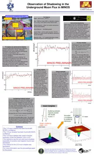
1. Observation of Shadowing in the Underground Muon Flux in MINOS Far Detector Depth – 2070 m.w.e. (700 m) Size – 5400 ton mass, 486 8 m diameter octagons, 31.5 m long. Every plane is fully instrumented. Passive Detector – Steel, for neutrino interactions and structural stability Active Detector – Scintillating plastic Cosmic Rays – 0.5 Hz cosmic ray rate. The Far Detector is a useful cosmic ray detector because of its size and depth. Magnetic Field – 1.5 T toroidal field allows charge sign determination for CPT studies, etc. Astronomical shadowing Optical astronomers use a catalogue of standard stars to calibrate their new instruments. Though there are no known cosmic ray sources, the sun and the moon are large enough to block a significant number of cosmic ray primaries and act as a calibration “standard sink”. They are close enough that the primaries that pass around each object aren’t bent back into its path by interplanetary magnetic fields nor the geomagnetic field. Since the moon’s location is well known, it can be used to find the absolute pointing and resolution of a particle detector. Special Thanks M. Kordosky 1-D moon shadow The plot at left is the one dimensional moon shadow, made using 20 million muons. The dashed red line is the Monte Carlo background and the solid curve is a Gaussian fit of form: where l is the average differential muon flux, s2 accounts for smearing from detector resolution, etc., and Rm = 0.26, the angular radius of the moon. The fit c2/ndof = 37.9/38, an improvement of 16.4 over the linear fit (54.3/39 a 10-4 chance probability) has parameters l = 483.9 ±3.1 and s2 = 0.34 ± 0.07. • To capture an astronomical shadow: • Eliminate data taken during times of detector problems (electronics, timing, calibration) • Eliminate muon tracks with poor pointing and resolution (reconstruction, etc.) • Find the location of the body using JPL’s Horizon’s database • Use the Haversine formula to find the 1-D separation of a particular muon from the body, (Dq), taking curvature into account. • Normalize each bin by the solid angle annulus given by the particular angular separation, according to: DWi=(2i-1)Sbin p, where Sbin = the square of bin size (0.01 deg2). 1-D sun shadow The plot at left is the one dimensional sun shadow. The dashed red line is the Monte Carlo background and the solid curve is a Gaussian fit. The fit c2/ndof = 40.3/38, an improvement of 8.2 over the liner fit (48.5/39 a 10-3 chance probability) has parameters l = 374.3 ±2.8 and s2 = 0.4 ± 0.09. The sun shadow is less significant than the moon because the sun is further away, allowing solar and interplanetary magnetic fields more time to bend muons back into the sun’s path. Charge separated In order to determine charge sign accurately, a cut on how well the reconstruction determined the momentum is required. This reduced the charge separated sample to 4.6 million muons, 2.7 positive and 1.9 negative. The plots at right are the charge separated one dimensional moon (top) and sun (bottom) shadow. The black triangles are positive, the red circles are negative, the dashed curve is the Gaussian fit, and the solid curve is the linear fit. The Gaussian fit offers little improvement over the linear fit for this sample because of such low statistics. The charge ratio for each distribution is 1.3. • Log-likelihood analysis method • Create a template of the expected shadow, using the known scattering of dimuons to simulate the effects of muons propagating through rock that affect shadowing. Compare the expected shape of the moon shadow centered at each 0.1o bin in Dd and DRA·cosd to the observed data. Sum over all bins in the shadow template: • Compare this sum to the no shadow hypothesis • See where the greatest deficit exists. This will give the absolute pointing of the detector by finding the most likely deficit in caused by the moon. This analysis is in progress; the method has been establishedand a result is forthcoming. moon template • Summary • The 1-D moon shadow has been found with 99.99% confidence • The 1-D sun shadow has been found with 99.9% confidence • The 1-D moon shadow was used to find the resolution of the Far Detector, 0.34 ± 0.07o • The method to see the sun and moon shadows separately for positive and negative muons was developed. • The method for the 2-D moon shadow was developed. • For more information see the proceedings paper for this poster. Special Thanks B.Bock, A. Habig This poster was supported directly by the U.S. Department of Energy. MINOS is supported by the U.S. Department of Energy and National Science Foundation, the U.K. Particle Physics and Astronomy Research Council, and the State and University of Minnesota.