Download
1 / 33
350 likes | 492 Vues
Lecture 9: NMR Theory and Instrumentation. Mass Spectrometry was very good at distinguishing many components of a mixture , but it was somewhat less good at telling us specifically what they were.

E N D
Lecture 9: NMR Theory and Instrumentation Mass Spectrometry was very good at distinguishing many components of a mixture, but it was somewhat less good at telling us specifically what they were. That’s because MS doesn’t give us any intramolecular information. Even if we bust our analyte up, we can only get molecular level information about the products In NMR the signals we observe depend on the environment of individual nuclei. Thus we can get information at the atomic level. Interestingly, though, we get less information about the whole molecule. NMR can have trouble distinguishing between a peptide that’s together and one that’s busted up!
NMR: The Instrument The first ‘bulk material’ NMR measurement was made by Purcell, Tory and Pound in 1945 on about 1 kg of paraffin wax. Since then, NMR technology has improved rapidly. NMR spectrometers now have the following general form: Probe. Holds sample close to tansmitter/ receiver coils LHe cooled superconducting persistent magnet. Our sample must be in a strong, homogeneous, stable magnetic field. RF transmitter capable of short, very high power ‘square’ pulses Receiver with very sensitive amplifier
NMR: The Chemical Shift Scale Firstly, NMR people have a strange way of describing magnets: They do it in MHz. The reason is that what you measure depends on the strength of the magnet. On a 500 MHz NMR, an unshielded proton will ‘precess’ at a frequency of 500 MHz. Differences in precession frequency due to electronic “shielding” are very small, on the order 100’s of Hz (.0001 MHz). To solve both of the above problems, we use a scale that is small (ppm) and relative to a reference compound (for H1 and C13 TMS). Due to the use of a reference compound, this scale is the same on every NMR instrument! frequency chemical shift
NMR and Energy Levels NMR is a spectroscopic method and is therefore subject to selection rules. The overriding selection rule is that we can only get useful signals from nuclei with a dipolar magnetic moment. This means that the quantum number mspin is either +1/2 or -1/2 This limits the nuclei we can use to (among others): 1H, 13C, 15N, 31P We can get signals from quadrupolar nuclei such as 2H.
NMR and Energy Levels In the absence of a magnetic field, spin states m+1/2 and m-1/2 (also called and or ‘up’ and ‘down’, respectively) have the same energy, thus the states will be populated equally When there is a magnetic field B0, the ‘spin state’ in which our dipolar magnet is ‘aligned’ with the field (we’ll say it’s ) is slightly lower in energy than the ‘un-aligned’ state . This description does not at all reflect reality, but we can now describe the energy of the states: Thus: Planck’s constant gyromagnetic ratio spin number Notice how small E is (h ≈ 6.6*10-34!). This is one way of explaining why NMR is so insensitive! magnetic field
Energy Levels and Scalar (J) Coupling The spin states and tell us the intensity of the NMR signal we are seeing, but they don’t tell us what we’re seeing If we’re sticking with our ‘energy levels’ description of NMR, then we need to say that there can be any number of and states (1, 2, 3, 1, 2, 3, etc.) each having a slightly different energy which we observe as a frequency. This is exactly analogous to other spectroscopic methods where we see peaks corresponding to specific energy transitions But in NMR, the energy of these transitions is affected by the energy of other nearby transitions through some kind of interaction. If the interaction is through a chemical bond, then it is called scalar or Jcoupling.
Scalar Coupling Scalar coupling is the reason for ‘peak splitting’ in NMR. For a system with two spins, we will not see a signal corresponding to a single spin, but a number of signals corresponding to all possible / combinations for the system: spins 1 and 2 are equivalent spins 1 is higher energy than spin 2 2 1 2 1 1 1 1 1 2 1 1 2 1 2 1 2 1 1 1 1 2 1 1 1 2 2 1 2 2 1 I I
The Vector Model The ‘energy levels’ picture can describe coupling, but it doesn’t really say anything about the signal we observe. Where do these frequencies come from? We said that the ‘’ state was aligned with the big magnetic field, but in reality this is only true as a bulk property of all the protons. They only tend to align themselves in such a way that their net magnetic vector is aligned… No Applied Magnetic Field (random) Applied Field (less random)
The Vector Model The transition to the ‘ state’ is also a bulk property and it is actually a flip 90° to the applied field (not 180°) z ? y x So now the field generated by the protons is 90° to the applied field and we should be able to measure it! Remember, our ity bity proton magnets were precessing, so the field they generate at 90° to the applied field is spinning on the xy plane. Even better! Because now we can measure frequencies!
Larmor Precession and the Rotating Frame So we have our magnetic field that is spinning on the xy plane. This field induces a tiny current in the receiver coils which we measure as a frequency The nuclei are spinning at their Larmor precession angular frequency, which is given by: But that is not what we measure. Because of how the NMR works, we measure 0 relative to a carrier frequency which we call the rotating frame. is called the offset frequency and that is the frequency that we measure in NMR
Getting to 90°: Resonance Our permanent magnet applies a powerful field. If we want to flip our nucleus generated field, say, onto the -y axis, we need to create a stronger field along the x axis…. but we can’t do that. Fortunately, there’s this little thing called resonance. Maybe the best way to think about this is to imagine the strength of magnetic field that would cause the nucleus to precess at the offset frequency: So if the carrier frequency rotfram is the same as the Larmor frequency 0, than = 0 and the effective field B = 0. When there is a small difference between rotfram and 0, the effective magnetic field – which is the field ‘felt’ by the nucleus - will be very small.
Getting to 90°: Hard Pulses So now we can cause the magnetic field derived from certain nucleito flip 90° with respect to the permanent magnetic field by using a transmitter to apply an RF field along x that oscillates at a frequency close to the appropriate 0. There are ‘scanning’ NMR instruments that work this way, but they are pretty much obsolete. The reason is that it’s much, much faster to excite all of the ‘amenable’ nuclei in the sample simultaneously. This gives us a complex wave function with lots of spins, but we know how to handle that!! (FT) To do this, we simply up the power of our RF field so that it can overpower B0 even at higher ||.
How Hard is Your Hard Pulse? The result is an excitation profile which describes, essentially, the range of offsets in which the effective fieldis overpowered by the applied field on x. Transmitter Frequency % ‘Flipped’ 100 50 -50 -100 0 (kHz) To derive the shape of these excitation profiles, we would need to solve the Bloch equations… but we won’t do that.
NMR: Working in Circles So we’ve used a hard pulse to get the magnetic field from our neuclei 90° to the z axis and onto -y. This magentic field is spining, so it actually goes from -y to x to y to -x (or vice versa, depending on the sign of the gyromagnetic ratio). It is spinning in the transverse plane. This shows the signal if we’re listening along the x or the y vector. Vector along which we are listening is called the receiver phase. Fundamentally, this is what we measure in NMR!
The Simplest NMR Experiment: Pulse Acquire We are now ready to look at our first real NMR experiment. This will constitute your introduction to ‘pulse sequence’ drawings. Pulse sequences are a series of RF pulses from the transmitter that are used to manipulate the induced magnetic field to do what we want. In this case, we want to ‘flip’ to 90° onto –y and then watch the result. z x -y x RF x rec -y
Pulses other than 90°: Flip Angles So far, we have carefully calibrated our RF pulse so that the induced magnetization goes on to the transverse plane For reasons that will become apparent later, we sometimes want to move our induced magnetization off of the transverse plane or ‘flip’ it to the other side of the transverse plane. We could do this by changing the power of our RF pulse, but it’s much easier and practical to change the duration. If we double the duration of our 90° (/2) pulse, we get a 180° () pulse; we flip the magnetization from +z to –z. If we are already in the transverse plane and we can use a 180° pulse to go from, say x to –x.
Refocusing Pulses: The Spin Echo Probably the second simplest NMR experiment is the ‘spin echo’. It has the following pulse sequence: The key thing about a pulse along one vector of the transverse plane (say x) is that it only affects the magnetization on the opposite vector x x RF 2 rec
Soft Pulses Sometimes we want to excite only a selected set of frequencies Obviously, we can do this by reducing the power of our RF pulse, and that is precisely what we do. ‘wiggles’ – these are bad We can eliminate the ‘wiggles’ (sortof) by using ‘shaped pulses’ (rather than a the ‘square’ on/off pulses we’ve been using so far). The simplest shape is a gaussian, but more complex shapes have been devised (e.g. REBURP)
Fourier Transforms and NMR Lineshape We’ve seen FT’s before, but in this case we need to be concerned about phase. We know the signal we’re looking at can be described by: This signal will decay exponentially over time, and we’re interested in the signal S, which is the absolute value of the magnetization so: We can combine these two components using complex numbers:
FTs and NMR Line Shape When we take our complex signal and fourier transform it, we get this: FT Absorption mode Dispersion Mode I I
Lineshape and Phase Error So our signal is some combination of absorption and dispersion mode lineshapes. To understand why it’s easier to think in the time domain: Of course we want to be able to extract a pure dispersion mode lineshape. To do this, we simply add a phase correction to our signal:
NMR and Quantum Mechanics We’ve now described NMR in two different ways that describe ‘parts’ of what we see. The only way to completely describe what goes on in NMR experiments is a rigorous quantum mechanical description… which we won’t do. But we still need to talk about things that neither the energy levels nor vector models can account for: Spin/Spin coupling and Spin Diffusion. These two phenomena are the basis for multidimensional NMR, which is a powerful analytical biochemistry tool! A 2D experiment is set up in the following general way: evolution t1 preparation mixing
Multidimesional NMR The preparation step is all about getting the magnetization where we want it so that when we leave it for a while (during t1) we get an antiphase term that reflects both coupled spins. We (usually) cannot generate an antiphase term by clever use of RF pulses. The antiphase term results only from the evolution of spins that are coupled. We need to give time t1 for this coupling to occur. Our antiphase term will result in a peak at 1 and 2, but only if the magnitization is on an observable axis (and has single quantum coherence). In the ‘mixing time’ we can use RF pulses to rotate the desired magnitizations onto the transverse plane
The 2D NMR Experiment What we actually do to measure 2D spectra is to measure a series of 1D spectra with increasingly longevolution periods. The phase of the absorption mode peak is oscillating! If we are looking at 1, this oscillation occurs at the ’s of all coupled spins!!
FTs and 2D NMR We now have a 2D wave function – one in the ‘direct dimension’ that oscillates at all ’s and one in the ‘indirect dimension’ that oscillates at all ’s coupled to each . FT(t2) FT(t1)
The Simplest 2D: COSY The COSY experiment has a very simple pulse sequence: x x Observe as: 1 in 12 in 2 Cross-peak! t1 Î1zÎ1-y Î1y Î2zÎ1zÎ2y Î1xÎ1x 12 22 Î1-yÎ1x Î1-yÎ1yÎ2z Observe as: 1 in 11 in 2 Diagonal peak! Antiphase term!! 2 11 21 Of course, we can do exactly the same for 2 1
Heteronuclear NMR So far, we’ve sortof assumed that 1 and 2 are the same type of nucleus. Heteronuclear NMR is quite similar except that we now need at least two transmitter channels to produce hard pulses at very different frequencies. The following is an INEPT sequence, which is commonly used to transfer magnetization from one nucleus to another: Transfer mag. from I to S Generate anti-phase, refocus offset Allow anti-phase to evolve to in phase y A version of this sequence is a ‘module’ in the HSQC experiment which links correlates N and H nuclei. I S
Relaxation When we’ve got our magnetization on the xy plane, there’s nothing keeping it there. In fact, the nuclei will, over time, reorient themselves so that the induced magnetic field returns to the z axis. This is called relaxation and, in general, it affects the width (or volume) of our NMR peaks. FT FT
Relaxation: Longitudinal and Transverse There are two types of relaxation: Longitudinal (T1) and Transverse (T2). Longitudinal relaxation occurs because after the RF pulse is finished, the B0 field is still there, making orientations aligned with the magnetic field lower energy. Thus, as nuclei change alignment, they will favor ‘B0 aligned’ alignments. The effect of longitudinal relaxation is to cause the induced magnetic field slow loose it’s ‘flip angle’ (initially 90°) . Transverse relaxation has two mechanisms: non-secular: interactions with local fields causes loss of transverse magnetization coherence secular: local field is very slightly different for each spin with ‘same’ . Over time, magnetization loses coherence.
Relaxation and Correlation Time The dominant mechanism of relaxation depends on the correlation timec of the analyte. In NMR, correlation time refers primarily to ‘rotational diffusion’ because this is the motion that is largely responsible with reorienting the nuclei with respect to B0. We won’t go into the details, but it turns out that T1 and T2 are similar at low c but diverge at high c. This actually causes one of the biggest drawbacks of biological NMR – we can’t use it on big proteins! TROSY is a pulse sequence module that helps deal with this issue somewhat
Phase Cycling So far, when we’ve looked at a pulse sequence, we’ve followed the magnetization through each pulse. But we’re forgetting something: What about unwanted magnetization from nuclei that are not coupled? For example, in the HSQC: not coupled coupled Some I may not be coupled to S y I I x/-x S I This is a very simple example of a phase cycle which are one of the reasons NMR experiments take so long
Gradients Using a ‘gradient’ means that you deliberately make the magentic field non-homogenious along one axis (usually z) Consequently, nuclei located at the lower (weak) end of the gradient will have lower 0 than nuclei at the upper (strong) end of the gradient Gradient pulses can have the effect of completely destroying coherence because they affect nuclei at different positions in the sample differently. 0 One trick to get rid of unwanted coherences is to get the one you do want onto z and then hit the sample with a z gradient pulse. This destroys all coherences except ones on z! This is called a ‘crusher gradient’
Gradients When you think about it, gradients can also provide positional information. You can measure the position of a nuclei with known by applying a field gradient and then using a soft pulse to excite one 0 at a time. Ever wonder how MRI’s work? Gradients are also used to ‘shim’ the NMR instrument. In the presence of a field gradient, a hard pulse will produce a broad, flat peak (because nuclei in different positions of the sample have different 0 and thus different ). If the magnetic field is not homogeneous along the z axis, the peak will be ‘bumpy’ because the imperfect field is resulting in an imperfect gradient.