Download
1 / 67
670 likes | 741 Vues
Explore a geostatistical model predicting water quality in stream segments using landscape-scale data. Learn about implications for water protection and compliance with environmental regulations. This research is funded by the U.S. EPA and presents a case study in Maryland. Discover methods, challenges, and solutions in monitoring stream conditions and spatial correlation analysis. Gain insights into geostatistical modeling, hydrologic distances, and assessing stream network configurations for improved predictions.

E N D
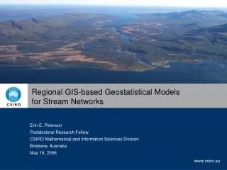
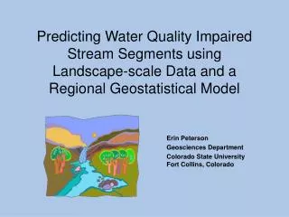
Predicting Water Quality Impaired Stream Segments using Landscape-scale Data and a Regional Geostatistical Model Erin Peterson Geosciences Department Colorado State UniversityFort Collins, Colorado
This research is funded by This research is funded by U.S.EPA U.S.EPA 凡 凡 Science To Achieve Science To Achieve Results (STAR) Program Results (STAR) Program Cooperative Cooperative CR CR - - 829095 829095 # # Agreement Agreement Space-Time Aquatic Resources Modeling and Analysis Program The work reported here was developed under STAR Research Assistance Agreement CR-829095 awarded by the U.S. Environmental Protection Agency (EPA) to Colorado State University. This presentation has not been formally reviewed by EPA. EPA does not endorse any products or commercial services mentioned in this presentation.
Overview Introduction ~ Background ~ Patterns of spatial autocorrelation in stream water chemistry ~ Predicting water quality impaired stream segments using landscape-scale data and a regional geostatistical model: A case study in Maryland
The Clean Water Act (CWA) 1972 Section 303(d) • Requires states and tribes to ID water quality impaired stream segments Section 305(b) • Create a biannual water quality inventory • Characterizes regional water quality • Based on attainment of designated-use standards assigned to individual stream segments
Probability-based Random Survey Designs • Used to meet section 305(b) requirements • Derive a regional estimate of stream condition • Assign a weight based on stream order • Provides representative sample of streams by order • Statistical inference about population of streams, within stream order, over large area • Reported in stream miles based on inference of attainment • Disadvantages • Does not take watershed influence into account • Does not ID spatial location of impaired stream segments • Fails to meet requirements of CWA Section 303(d)
Purpose Develop a geostatistical methodology based on coarse-scale GIS data and field surveys that can be used to predict water quality characteristics about stream segments found throughout a large geographic area (e.g., state)
SCALE: Grain Aquatic Terrestrial Landscape River Network COARSE Climate Atmospheric deposition Geology Topography Soil Type Network Connectivity Stream Network Nested Watersheds Drainage Density Confluence Density Connectivity Flow Direction Network Configuration Vegetation Type Basin Shape/Size Land Use Topography Segment Contributing Area Segment Tributary Size Differences Network Geometry Localized Disturbances Land Use/ Land Cover Reach Riparian Zone Riparian Vegetation Type & Condition Floodplain / Valley Floor Width Cross Sectional Area Channel Slope, Bed Materials Large Woody Debris Overhanging Vegetation Substrate Microhabitat Microhabitat FINE Biotic Condition, Substrate Type, Overlapping Vegetation Detritus, Macrophytes Shading Detritus Inputs Biotic Condition
10 Sill Semivariance Nugget Range 0 1000 0 Separation Distance Geostatistical Modeling • a.k.a. Kriging • Interpolation method • Allows spatial autocorrelation in error term • More accurate predictions • Fit an autocovariance function to data • Describes relationship between observations based on separation distance • 3 Autocovariance Parameters • Nugget: variation between sites as separation distance approaches zero • Sill: delineated where semivariance asymptotes • Range: distance within which spatial autocorrelation occurs
B A C Distance Measures & Spatial Relationships Distances and relationships are represented differently depending on the distance measure Straight-line Distance (SLD) Geostatistical models typically based on SLD
B A C Distance Measures & Spatial Relationships Distances and relationships are represented differently depending on the distance measure Symmetric Hydrologic Distance (SHD) Hydrologic connectivity: Fish movement
B A C Distance Measures & Spatial Relationships Distances and relationships are represented differently depending on the distance measure Asymmetric Hydrologic Distance Longitudinal transport of material
B A C Distance Measures & Spatial Relationships Distances and relationships are represented differently depending on the distance measure • Challenge: • Spatial autocovariance models developed for SLD may not be valid for hydrologic distances • Covariance matrix is not positive definite
Flow Asymmetric Autocovariance Models for Stream Networks • Weighted asymmetric hydrologic distance (WAHD) • Developed by Jay Ver Hoef, National Marine Mammal Laboratory, Seattle • Moving average models • Incorporate flow volume, flow direction, and use hydrologic distance • Positive definite covariance matrices Ver Hoef, J.M., Peterson, E.E., and Theobald, D.M., Spatial Statistical Models that Use Flow and Stream Distance, Environmental and Ecological Statistics. In Press.
Patterns of Spatial Autocorrelation in Stream Water Chemistry
Objectives Evaluate 8 chemical response variables • pH measured in the lab (PHLAB) • Conductivity (COND) measured in the lab μmho/cm • Dissolved oxygen (DO) mg/l • Dissolved organic carbon (DOC) mg/l • Nitrate-nitrogen (NO3) mg/l • Sulfate (SO4) mg/l • Acid neutralizing capacity (ANC) μeq/l • Temperature (TEMP) °C Determine which distance measure is most appropriate • SLD • SHD • WAHD • More than one? Find the range of spatial autocorrelation
Dataset Maryland Biological Stream Survey (MBSS) Data • Maryland Department of Natural Resources • 1995, 1996, 1997 • Stratified probability-based random survey design • 881 sites in 17 interbasins
Maryland Baltimore Annapolis Northeastern U.S. Washington D.C. Chesapeake Bay Study Area
N Spatial Distribution of MBSS Data
2 1 3 1 2 3 1 2 3 SHD AHD SLD GIS Tools Automated tools needed to extract data about hydrologic relationships between survey sites did not exist! Wrote Visual Basic for Applications (VBA) programs to: • Calculate watershed covariates for each stream segment • Functional Linkage of Watersheds and Streams (FLoWS) • Calculate separation distances between sites • SLD, SHD, Asymmetric hydrologic distance (AHD) • Calculate the spatial weights for the WAHD • Convert GIS data to a format compatible with statistics software • FLoWS tools will be available on the STARMAP website: • http://nrel.colostate.edu/projects/starmap
Calculate the PI of each upstream segment on segment directly downstream Watershed Segment B Watershed Segment A • Calculate the PI of one survey site on another site • Flow-connected sites • Multiply the segment PIs A B C Watershed Area A Segment PI of A = Watershed Area B Spatial Weights for WAHD • Proportional influence (PI): influence of each neighboring survey site on a downstream survey site • Weighted by catchment area: Surrogate for flow volume
Calculate the PI of each upstream segment on segment directly downstream A C B • Calculate the PI of one survey site on another site • Flow-connected sites • Multiply the segment PIs E D F G H Spatial Weights for WAHD • Proportional influence (PI): influence of each neighboring survey site on a downstream survey site • Weighted by catchment area: Surrogate for flow volume survey sites stream segment
Calculate the PI of each upstream segment on segment directly downstream • Calculate the PI of one survey site on another site • Flow-connected sites • Multiply the segment PIs Site PI = B * D * F * G Spatial Weights for WAHD • Proportional influence (PI): influence of each neighboring survey site on a downstream survey site • Weighted by catchment area: Surrogate for flow volume A C B E D F G H
Data for Geostatistical Modeling • Distance matrices • SLD, SHD, AHD • Spatial weights matrix • Contains flow dependent weights for WAHD • Watershed covariates • Lumped watershed covariates • Mean elevation, % Urban • Observations • MBSS survey sites
Geostatistical Modeling Methods • Validation Set • Unique for each chemical response variable • 100 sites • Initial Covariate Selection • Reduce covariates to 5 • Model Development • Restricted model space to all possible linear models • Model set = 32 models (25 models) • One model set for: • General linear model (GLM), SLD, SHD, and WAHD models
Log-likelihood function of the parameters ( ) given the observed data Z is: Maximizing the log-likelihood with respect to B and sigma2 yields: and Both maximum likelihood estimators can be written as functions of alone Derive the profile log-likelihood function by substituting the MLEs ( ) back into the log-likelihood function Geostatistical Modeling Methods • Geostatistical model parameter estimation • Maximize the profile log-likelihood function
where is the covariance based on the distance between two sites, D, given the covarianceparameter estimates: nugget ( ), sill ( ), and range ( ). Geostatistical Modeling Methods Fit exponential autocorrelation function • Model selection within model set • GLM: Akaike Information Corrected Criterion (AICC) • Geostatistical models: Spatial AICC (Hoeting et al., in press) where n is the number of observations, p-1 is the number of covariates, and k is the number of autocorrelation parameters. http://www.stat.colostate.edu/~jah/papers/spavarsel.pdf
Geostatistical Modeling Methods • Model selection between model types • 100 Predictions: Universal kriging algorithm • Mean square prediction error (MSPE) • Cannot use AICC to compare models based on different distance measures • Model comparison: r2 for observed vs. predicted values
Summary statistics for distance measures in kilometers using DO (n=826). * Asymmetric hydrologic distance is not weighted here Results • Summary statistics for distance measures • Spatial neighborhood differs • Affects number of neighboring sites • Affects median, mean, and maximum separation distance
180.79 301.76 SLD SHD WAHD Results Mean Range Values SLD = 28.2 km SHD = 88.03 km WAHD = 57.8 km • Range of spatial autocorrelation differs: • Shortest for SLD • TEMP = shortest range values • DO = largest range values
GLM SLD MSPE SHD WAHD Results • Distance Measures: • GLM always has less predictive ability • More than one distance measure usually performed well • SLD, SHD, WAHD: PHLAB & DOC • SLD and SHD : ANC, DO, NO3 • WAHD & SHD: COND, TEMP • SLD distance: SO4
r2 GLM SLD SHD WAHD Results Predictive ability of models: Strong: ANC, COND, DOC, NO3, PHLAB Weak: DO, TEMP, SO4 r2
SHD WAHD SLD Discussion Distance measure influences how spatial relationships are represented in a stream network • Site’s relative influence on other sites • Dictates form and size of spatial neighborhood • Important because… • Impacts accuracy of the geostatistical model predictions
Patterns of spatial autocorrelation found at relatively coarse scale • Geostatistical models describe more variability than GLM SLD, SHD, and WAHD represent spatial autocorrelation in continuous coarse-scale variables SLD • > 1 distance measure performed well • SLD never substantially inferior • Do not represent movement through network • Different range of spatial autocorrelation? • Larger SHD and WAHD range values • Separation distance larger when restricted to network SHD
244 sites did not have neighbors Sample Size = 881 Number of sites with ≤1 neighbor: 393 Mean number of neighbors per site: 2.81 Frequency Number of Neighboring Sites Discussion • Probability-based random survey design (-) affected WAHD • Maximize spatial independence of sites • Does not represent spatial relationships in networks • Validation sites randomly selected
4500 WAHD GLM Difference 0 0 1 2 3 4 5 6 7 9 10 11 12 13 14 15 16 17 8 Number of Neighboring Sites Discussion WAHD models explained more variability as neighboring sites increased • Not when neighbors had: • Similar watershed conditions • Significantly different chemical response values
4500 WAHD GLM Difference 0 0 1 2 3 4 5 6 7 9 10 11 12 13 14 15 16 17 8 Number of Neighboring Sites Discussion • GLM predictions improved as number of neighbors increased • Clusters of sites in space have similar watershed conditions • Statistical regression pulled towards the cluster • GLM contained hidden spatial information • Explained additional variability in data with > neighbors
Coarse COND SO4 ANC PH NO3 DOC Scale of dominant ecological processes TEMP DO Fine 0.5 0 1.0 Predictive Ability of Geostatistical Models r2
Conclusions • Spatial autocorrelation exists in stream chemistry data at a relatively coarse scale • Geostatistical models improve the accuracy of water chemistry predictions • Patterns of spatial autocorrelation differ between chemical response variables • Ecological processes acting at different spatial scales • SLD is the most suitable distance measure at regional scale at this time • Unsuitable survey designs • SHD: GIS processing time is prohibitive
Conclusions • Results are scale specific • Spatial patterns change with survey scale • Other patterns may emerge at shorter separation distances • Further research is needed at finer scales • Watershed or small stream network • Need new survey designs for stream networks • Capture both coarse and fine scale variation • Ensure that hydrologic neighborhoods are represented
Predicting Water Quality Impaired Stream Segments using Landscape-scale Data and a Regional Geostatistical Model: A Case Study In Maryland
Objective Demonstrate how a geostatistical methodology can be used to meet the requirements of the Clean Water Act • Predict regional water quality conditions • ID the spatial location of potentially impaired stream segments
1996 MBSS DOC Data Kilometers 0 20 N
Methods Potential covariates
Methods Potential covariates after initial model selection (10)
Methods • Fit geostatistical models • Two distance measures: SLD and WAHD • Restricted model space to all possible linear models • 1024 models per set (210 models) • Parameter Estimation • Maximized the profile log-likelihood function
Model selection within distance measure & autocorrelation function • Spatial AICC (Hoeting et al., in press) Model selection between distance measure & autocorrelation function • Cross-validation method using Universal kriging algorithm • 312 predictions • MSPE • Model comparison: r2 for the observed vs. predicted values Methods
MSPE Mariah Linear with Sill Rational Quadratic Spherical Exponential Hole Effect Autocorrelation Function Results • SLD models performed better than WAHD • Exception: Spherical model • Best models: • SLD Exponential, Mariah, and Rational Quadratic models • r2 for SLD model predictions • Almost identical • Further analysis restricted to SLD Mariah model
Results • Covariates for SLD Mariah model: • WATER, EMERGWET, WOODYWET, FELPERC, & MINTEMP • Positive relationship with DOC: • WATER, EMERGWET, WOODYWET, MINTEMP Negative relationship with DOC • FELPERC
Model coefficients represent change in log10 DOC per unit of X Cross-validation intervals for Mariah model regression coefficients • Cross-validation interval: 95% of regression coefficients produced by leave-one-out cross validation procedure • Narrow intervals • Few extreme regression coefficient values • Not produced by common sites • Covariate values for the site are represented in observed data • Not clustered in space
r2 Observed vs. Predicted Values 1 influential site r2 without site = 0.66 n = 312 sites r2 = 0.72