Chapter 3 Mobile Radio Propagation
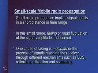
550 likes | 1.1k Vues
Chapter 3 Mobile Radio Propagation. 曾志成 國立宜蘭大學 電機工程學系 tsengcc@niu.edu.tw. Speed, Wavelength, Frequency. Light Speed ( c ) = Wavelength ( l ) x Frequency ( f ) = 3 10 8 m/s. Types of Radio Waves. Ionosphere ( 80 - 720 km). 電離層. Sky wave.

Chapter 3 Mobile Radio Propagation
E N D
Presentation Transcript
Chapter 3Mobile Radio Propagation 曾志成 國立宜蘭大學 電機工程學系 tsengcc@niu.edu.tw EE of NIU
Speed, Wavelength, Frequency • Light Speed (c) = Wavelength (l) x Frequency (f) = 3 108m/s EE of NIU
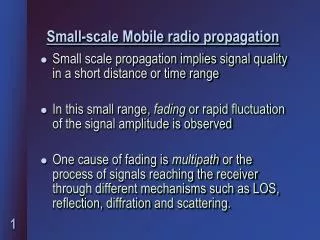
Types of Radio Waves Ionosphere (80 - 720 km) 電離層 Sky wave Mesosphere (50 - 80 km) 中氣層 平流層 Stratosphere (12 - 50 km) Space wave (LOS) Ground wave 對流層 Troposphere (0 - 12 km) Transmitter Receiver Earth EE of NIU
Radio Frequency Bands EE of NIU
Propagation Mechanisms • Reflection (反射) • Propagation wave impinges on an object which is large as compared to wavelength, e.g., the surface of the Earth, buildings, walls, etc. • Diffraction(繞射) • Radio path between transmitter and receiver obstructed by surface with sharp irregular edges, e.g., waves bend around the obstacle, even when LOS (line of sight) does not exist. • Scattering(散射) • Objects smaller than the wavelength of the propagation wave, e.g. foliage, street signs, lamp posts. EE of NIU
Radio Propagation Effects EE of NIU
Free-Space Propagation • Assuming that the radiated power is uniformly distributed over the surface of the sphere. • The received signal power at distance d: • Pt is transmitting power • Ae is effective areacovered by the sender • Gt is the transmitting antenna gain EE of NIU
Antenna Gain • For a circular reflector antenna, the antenna gain • is the net efficiency (typically 0.55) • D is the diameter • c is the speed of light 3108 m/s • Example: • If the antenna diameter = 2 m and frequency = 6 GHz, then, wavelength = 0.05 m and G = 39.4 dB. • If the frequency = 14 GHz and diameter = 2 m , then, the wavelength = 0.021 m and G = 46.9 dB • Higher the frequency, higher the gain for the same size antenna. EE of NIU
Land Propagation • The received signal power: • Gr is the receiver antenna gain, • L is the propagation loss in the channel, i.e., L = LP LS LF Fast fading Slow fading Path loss EE of NIU
Path Loss (Free-Space) • Definition of path loss LP : • The signal strength decays exponentially with distance d between transmitter and receiver; • The loss could be proportional to somewhere between d2 and d4 depending on the environment. • Path Loss in Free-space: • fc is the carrier frequency. • This shows greater the fc, more is the loss. EE of NIU
Path Loss (Land Propagation) • Simplest Formula: • A and α are the propagation constants • d is the distance between transmitter and receiver • α is the value of 3 ~ 4 in typical urban area EE of NIU
Example of Path Loss (Free-space) EE of NIU
Path Loss in Different Areas (1) • Path loss in decreasing order: • Urban area (large city) • Urban area (medium and small city) • Suburban area • Open area EE of NIU
Path Loss in Different Areas (2) • Urban Area where • For a large city, the path loss is the same as the that for small- and medium cities under hb=50m and hm=1.65m. correction factor for the mobile antenna height EE of NIU
Concept Used for Calculating a(hm) hb hm Distance d Transmitter Receiver EE of NIU
Path Loss in Different Areas (3) • Suburban • Open area 課本(3.14)式有誤 EE of NIU
Path Loss --- Urban: Large City hb=50m and hm=1.65m EE of NIU
Path Loss --- Urban: Medium and Small Cities hb=50m and hm=1.65m EE of NIU
Path Loss --- Suburban Area hb=50m and hm=1.65m EE of NIU
Path Loss --- Open Area hb=50m and hm=1.65m EE of NIU
Fading Fast Fading (Short-term fading) Slow Fading (Long-term fading) Signal Strength (dB) Path Loss Distance EE of NIU
Slow Fading • What is slow fading? • Long-term variation in the mean level of received signals. • The channel impulse response changes at a rate much slower than the transmitted baseband signal. • Slow fading is also called shadowing or log-normal fading because its amplitude has a log-normal pdf. • The amplitude change caused by shadowing is often modeled using a log-normal distribution. EE of NIU
Shadowing • Log-normal distribution • The pdf of the received signal level is given in decibels by • M is the true received signal level m in decibels, i.e., 10log10m. • is the area average signal level, i.e., the mean of M. • is the standard deviation in decibels. EE of NIU
Log-normal Distribution 2 p(M) M M EE of NIU
Fast Fading • What is fast fading? • Short-term fading due to fast spatial variation. • The channel impulse response changes rapidly than the transmitted baseband signal. EE of NIU
Fast Fading --- Receiver Far From the Transmitter • Assume • There are no direct radio waves between transmitter and receiver. • The prob. distribution of signal amplitude of every path is a Gaussian distribution. • The phase distribution of every path is uniformly distributed over (0,2p) radians. • The prob. distribution of the envelope for the composite signals is a Rayleigh distribution. EE of NIU
P(r) 1.0 0.8 =1 0.6 =2 0.4 =3 0.2 r 0 2 6 10 4 8 Rayleigh Distribution ris the envelope of the fading signal sis the standard deviation EE of NIU
Fast Fading --- Receiver Close to the Transmitter • Assume • The direct radio wave between transmitter and receiver is stronger than other radio waves. • The prob. distribution of signal amplitude of every path is a Gaussian distribution. • The phase distribution of every path is uniformly distributed over (0,2p) radians. • The prob. distribution of the envelope for the composite signals is a Rician distribution. EE of NIU
Rician Distribution b= 0 (Rayleigh) = 1 b = 1 b = 2 b = 3 ris the envelope of the fading signal sis the standard deviation bis the amplitude of the direct signal I0(x)is the zero-order Bessel function of the first kind Pdf p(r) r EE of NIU
General Model of Fading Channel --- Nakagami • For Nakagami distribution, the pdf of the received signal envelop is • is the Gamma function • is the average power, i.e., the 2nd moment of the fading signal is the fading term, where m≥ 0.5 • If m=1, Nakagami distribution becomes to Rayleigh distribution • If m approach to infinity, the distribution becomes to an impulse, i.e., no fading. • Nakagami is used to replace Rician since Bessel function is not required EE of NIU
Characteristics of Instantaneous Amplitude • Level Crossing Rate: • Average number of times per second that the signal envelope crosses a specified level in positive going direction. • Fading Rate: • Number of times signal envelope crosses middle value in positive going direction per unit time. • Depth of Fading: • Ratio of mean square value and minimum value of fading signal. • Fading Duration: • Time for which signal is below given threshold. EE of NIU
Doppler Effect • When a wave source and a receiver are moving, the frequency of the received signal will not be the same as the source. • When they are moving toward each other, the frequency of the received signal is higher than the source. • When they are opposing each other, the frequency decreases. • The frequency of the received signal is • fC is the frequency of source carrier, • fD is the Doppler frequency. EE of NIU
Doppler Shift • Doppler frequency (or Doppler shift) • v is the moving speed, • is the wavelength of carrier q MS Moving direction of receiver with speed v Signal from sender EE of NIU
Moving Speed Effect V1 V2 V3 V4 Signal strength Time EE of NIU
Delay Spread • When a signal propagates from a transmitter to a receiver, signal suffers one or more reflections. • This forces signal to follow different paths. • Each path has different path length, so the time of arrival for each path is different. • This effect which spreads out the signal is called “Delay Spread”, td. EE of NIU
Delay Spread The signals from close by reflectors The signals from intermediate reflectors Signal Strength The signals from far away reflectors Delay EE of NIU
Inter-Symbol Interference (ISI) • Caused by time delayed multipath signals • Has impact on burst error rate of the channel • If the transmission rate is R, a low bit-error-rate (BER) can be obtained when EE of NIU
Inter-Symbol Interference (ISI) Transmission signal 1 1 Time 0 Received signal (short delay) Time Propagation time Delayed signals Received signal (long delay) Time EE of NIU
Coherence Bandwidth • Coherence bandwidth Bc≈ 1/(2πd) • A statistical measure of the range of frequencies over which the channel can be considered as “flat”. • Flat fading • If the bandwidth of Tx signal is lower than the channel coherent bandwidth, nonlinear transformation could no occur. • Frequency-selective fading • If the bandwidth of Tx signal is higher than the channel coherent bandwidth, nonlinearity is present. EE of NIU
Cochannel Interference • Cells having the same frequency interfere with each other. • In a cellular system, to reuse the frequencies, the same frequency is assigned to different cells. EE of NIU
Homework • P3.1 • P3.2 • P3.4 • P3.5 • P3.7 • P3.14 EE of NIU