Mobile Radio Propagation
810 likes | 1.2k Vues
Mobile Radio Propagation. Mobile radio channel is an important factor in wireless systems. Wired channels are stationary and predictable, while radio channels are random and have complex models . Modeling of radio channels is done in statistical fashion based on receiver measurements.

Mobile Radio Propagation
E N D
Presentation Transcript
Mobile Radio Propagation • Mobile radio channel is an important factor in wireless systems. • Wired channels are stationary and predictable, while radio channels are random and have complex models. • Modeling of radio channels is done in statistical fashion based on receiver measurements.
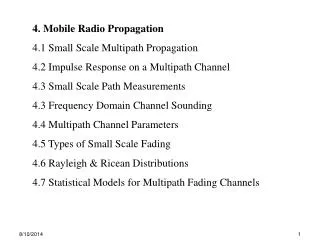
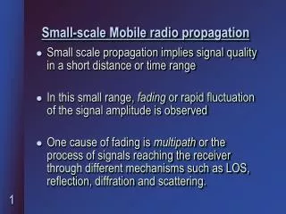
Types of propagation models • Large scale propagation models • To predict the averagesignal strength at a given distance from the transmitter • Controlled by signal decay with distance • Small scale or fading models. • To predict the signal strength at close distance to a particular location • Controlled by multipath and Doppler effects.
-30 -40 Received Power (dBm) -50 -60 -70 14 16 18 20 22 24 26 28 T-R Separation (meters) Radio signal pattern
Measured signal parameters • Electrical Field (Volts/m) Magnitude E = IEI Vector Direction E = xEx + yEy + zEz • Power (Watts or dBm) Power is scalar quantity and easier to measure.
Relation between Watts and dBm • P (dBm) = 10 log10 [P(mW)]
Physical propagation models • Free Space Propagation • Transmitter/receiver have clear LOS path • Reflection • Wave reaches receiver after reflection off surfaces larger than wavelength • Diffraction • Wave reaches receiver by bending at sharp edges (peaks) or curved surfaces (earth). • Scattering • Wave reaches receiver after bouncing off objects smaller than wavelength (snow, rain).
Free Space Propagation • Transmitter and receiver have clear, unobstructed LOS path between them. (Courtesy: webbroadband.blogspot.com)
Friistransmission equation Pr = PtGt Gr2 (4)2 d2 L Pt= Transmitted Power (W) Pr = Received Power (W) Gt= Transmitter antenna gain Gr = Receiver antenna gain L = System loss factor • Due to line losses, but not due to propagation • L 1
Antenna Gain • Power Gain of antenna G = 4Ae / 2, • Ae is effective aperture area of antenna • Wavelength = c / f (Hz) = 3 • 108 / f , meters
Relation between Electric field and Power • Received power Pr= IErI2 2 Gr 4 • Impedance of medium: = / • For air or vacuum: = (4 • 10-7) /(8.85 • 10-12 ) = 377
Example If the received power is Pr = 7 • 10-10 W, antenna gain Gr = 2 and transmitting frequency is 900 MHz, determine the electric field strength at the receiver.
Solution f = 900 MHz => = (3 • 108) / (900 • 106) = 0.33 m From field-power equation: IErI = [(Pr • • 4) / ( 2 • Gr)]1/2 = [(7 • 10-10• 377 • 4) / (0.332 • 2)]1/2 = 0.0039 V/m
Example A transmitter produces 50W of power. If this power is applied to a unity gain antenna with 900 MHz carrier frequency, find the received power at a LOS distance of 100 m from the antenna. What is the received power at 10 km? Assume unity gain for the receiver antenna.
Solution Pr = PtGt Gr2 (4)2 d2 L Pt = 50 W, Gt = 1, Gr = 1, L = 1, d = 100 m = (3 • 108) / (900 • 106) = 0.33 m Solving, Pr = 3.5 • 10-6 W Pr (10 km) = Pr (100 m) • (100/10000)2 = 3.5 • 10-6 • (1/100)2 = 3.5 • 10-10 W
Electric Properties of Material Bodies • Fundamental constants Permittivity = 0r , Farads/m Permeability = 0r ,Henries/m Conductivity ,Siemens/m • Types of materials • Dielectrics – allow EM waves to pass • Conductors – block EM waves • Metamaterials – bend EM waves
Reflection at dielectric boundaries Er = : Reflection coefficient Et = T = 1 + : Transmission coefficient Ei Ei Er Ei i r i= r Et
Vertical Polarization Ei Er Hi Hr 1, 1, 1 i r 2, 2, 2 t Et ||= 2sint - 1sini 2sint + 1sini
Horizontal Polarization Ei Er Hi Hr 1, 1, 1 i r 2, 2, 2 t Et T = 2sint - 1sini 2sint + 1sini
Reflection from Perfect Conductor (ET =0) Vert. polarizationHoriz. polarization i=ri=r Ei = ErEi = - Er Ei Er i r Et
Ground Reflection (2-Ray Model) T (transmitter) ETOT = ELOS +Eg ELOS Ei R (receiver) ht Er=Eg hr i 0 d
Field Equations d = several kms ht = 50-100m ETOT= ELOS + Eg ETOT(d) = For d > 20hthr / Received power Pr=
Example A mobile is located 5 km away from a base station, and uses a vertical /4 monopole antenna with a gain of 2.55dB to receive cellular radio signals. The electric field at 1 km from the transmitter is measured to be 10-3 V/m. The carrier frequency used is 900 MHz. (a) Find the length and gain of the receiving antenna.
Example A mobile is located 5 km away from a base station, and uses a vertical /4 monopole antenna with a gain of 2.55dB to receive cellular radio signals. The electric field at 1 km from the transmitter is measured to be 10-3 V/m. The carrier frequency used is 900 MHz. (b) Find the received power at the mobile using the 2-way ground model assuming the height of the transmitting antenna is 50 m and receiving antenna is 1.5 m above the ground.
Solution: d0 = 1 km E0 = 10-3 V/m ht = 50 m hr = 1.5 m d = 5 km
(a) f = 900 MHz = (3 • 108) / (900 • 106) = 0.33 m Length of receiving antenna, L = / 4 = 0.33/4 = 0.0833 m = 8.33 cm
(b) Gain of antenna = 2.55 dB = > 1.8 Er (d) = = 2 • 10-3 • 1 • 103 • 2 • 50 • 1.5 (5 • 103)2 • 0.333 = 113.1 • 10-6 V/m
Pr (d) = I Er I22 Gr 4 = (113.1 • 10-6) 2 • (0.333) 2 • 1.8 377 4 = 5.4 • 10-13 W = -92.68 dBm
Diffraction • Diffraction allows radio signals to propagate around the curved surface or propagate behind obstructions. • Based on Huygen’s principle of wave propagation.
R T h d2 d1 ht hr hobs Knife-edge Diffraction Geometry (a) T is transmitter and R is receiver, with an infinite knife-edge obstruction blocking the line-of-sight path.
T h h’ R d1 d2 ht hr Knife-edge Diffraction Geometry (b) T & R are not the same height...
T h h’ R d1 d2 ht hr Knife-edge Diffraction Geometry ...If and are small and h<<d1 and d2, then h & h’ are virtually identical and the geometry may be redrawn as in (c).
Knife-edge Diffraction Geometry (c) Equivalent where the smallest height (in this case hr ) is subtracted from all other heights. T ht-hr hobs-hr R d2 d1
Assumptions h << d1, d2 h >> Excess path length
...Assumptions h << d1, d2 h >> Phase difference = 2 / = 2 h2 (d1 + d2 ) 2 d1 d2
Diffraction Parameter v = =
Three Cases • Case I: h > 0 • Case II: h = 0 • Case III: h < 0
Case I: h > 0 and are positive since h is positive. h T R d1 d2
Case II: h = 0 and equal 0, since h equals 0. d1 d2 T R
Case III: h < 0 and are negative, since h is negative. d1 d2 T R h
The electric field strength of the diffracted wave is given by: Ed = F(v) • Eo where Eois the free space field strength in the absence of both ground and knife edge.
Approximate Value of Fresnel Integral F(v): Gd(dB) = 20log IF(v)I
v Range Gd (dB) v -1 0 -1v 0 20 log (0.5 – 0.62 v) 0v1 20 log (0.5 e-0.95v) 1v2.4 20 log (0.4 – v2.4 20 log (0.225 /v)
Example Compute the diffraction loss between the transmitter and receiver assuming: = 1/3m d1 = 1km d2 = 1km h = 25m
Solution: Given = 1/3 m d1 = 1km d2 = 1km h = 25m V = = = 2.74
Using the table, Gd (dB) = 20 log (0.225/2.74) = -22 dB Loss = 22 dB
Scattering • When a radio wave impinges on a rough surface, the reflected energy is spread out or diffused in all directions. Ex., lampposts and foliage. • The scattered field increases the strength of the signal at the receiver.
Radar Cross Section (RCS) Model RCS (Radar Cross Section) = Power density of scattered wave in direction of receiver Power density of radio wave incident on the scattering object
Radar Cross Section (RCS) Model PR = PT • GT • 2 • RCS (4)3 • dT 2 • dR 2 Where, PT = Transmitted Power GT = Gain of Transmitting antenna dT = Distance of scattering object from Transmitter dR = Distance of scattering object from Receiver
Practical Link Budget • Most radio propagation models are derived using a combination of analytical and empirical models. • Empirical approach is based on fitting curves or analytical expressions that recreate a set of measured data.
...Practical Link Budget • Advantages of empirical models; Takes into account all propagation factors, both known and unknown. • Disadvantages:New models need to be measured for different environment or frequency.