Mobile Radio Propagation

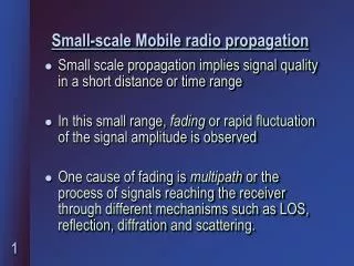
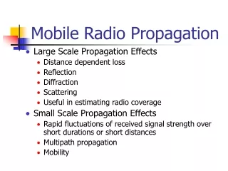
1. Mobile Radio Propagation • Large Scale Propagation Effects • Distance dependent loss • Reflection • Diffraction • Scattering • Useful in estimating radio coverage • Small Scale Propagation Effects • Rapid fluctuations of received signal strength over short durations or short distances • Multipath propagation • Mobility

2. Propagation Scenario

3. Propagation phenomena

4. Large-scale /small-scale propagation

5. 1 – 2 Km 50-100

6. Free space propagation model - LOS • Assumes far-field (Fraunhofer region) • Far field distance df >> D and df >>  , where • D is the largest linear dimension of antenna •  is the carrier wavelength • df = 2D2/  • No interference, no obstructions • Effective isotropic radiated power – EIRP = Pt Gt dBi • Effective radiated power – ERP dBd • Pr= Pt Gt Gr 2/ (4d)2 L  Pt(d0/d)2 • do > df Fraunhofer region/far field (1m -1 km) • Path loss PL(dB) = 10log (Pt/Pr)

7. Radio Propagation Mechanisms • Reflection • Propagating EM wave impinges on an object which is large as compared to its wavelength - e.g., the surface of the Earth, buildings, walls, etc. • Conductors & Dielectric materials (refraction) • Diffraction • Radio path between transmitter and receiver is obstructed by a surface with sharp irregular edges • Waves bend around the obstacle, even when LOS (line of sight) does not exist • Fresnel zones • Scattering • Objects smaller than the wavelength of the propagating wave - e.g. foliage, street signs, lamp posts • “Clutter” is small relative to wavelength

8. Reflection • Perfect conductors reflect with no attenuation • Light on the mirror • Dielectrics reflect a fraction of incident energy • “Grazing angles” reflect max* • Steep angles transmit max* • Light on the water • Reflection induces 180 phase shift • Why? See yourself in the mirror • Reflected field intensity • Fresnel reflection coefficient  • Brewster angle   = 0 ? q qr qt

9. Classical 2-ray Ground reflection model

10. 2-Ray Model • E(d,t) = (Eodo/d) cos { c(t – d/c)} ; d>do • ELOS(d’,t) = (Eodo/d’) cos { c(t – d’/c)} • Eg(d’’,t) =  (Eodo/d’’) cos { c(t – d’’/c)} • i = o  Eg =  Ei ; Et = (1+) Ei • Assuming perfect horizontal E-field polarization and ground reflection , | =-1, Et = 0 • |ETOT| = |ELOS + Eg | • ETOT(d,t) = (Eodo/d’) cos { c(t – d’/c)} +(-1)(Eodo/d’’) cos { c(t – d’’/c)}

11. Method of images

12. 2-Ray model • Using method of images, • Path difference  = d’’ – d’ = {(ht+hr)2+d2} 1/2 –{(ht-hr)2+d2} 1/2 • If d >> (ht+hr) ;  = d’’ – d’  2hthr /d •  = 2 /  =  c / c and d = / c = /2 fc • At time t = d’’/c ; • ETOT(d, t) = (Eodo/d’) cos { c((d’’ – d’)/c) - (Eodo/d’’) cos 0 = (Eodo/d’)   - (Eodo/d’’)  (Eodo/d) [   - 1] • |ETOT(d) |= { (Eodo/d)2 cos ( - 1)2 + (Eodo/d)2 sin ( )2 } ½

13. 2-Ray model • |ETOT(d) |= { (Eodo/d)2 cos ( - 1)2 + (Eodo/d)2 sin ( )2 } ½ • |ETOT(d) |= (Eodo/d) (2-2cos  ) ½ = (2Eodo/d) sin(  /2) • sin(  /2)  (  /2) < 0.3 rad  d > 20 ht hr /  • ETOT(d)  (2Eodo/d) (2  ht hr / d)  k / d 2 V/m • Pr= Pt Gt Gr (ht hr)2/ d 4 • PL(dB) = 40 log d – ( 10logGt + 10logGr + 20loght + 20loghr )

14. Diffraction Diffraction occurs when waves hit the edge of an obstacle “Secondary” waves propagated into the shadowed region Water wave example Diffraction is caused by the propagation of secondary wavelets into a shadowed region. Excess path length results in a phase shift The field strength of a diffracted wave in the shadowed region is the vector sum of the electric field components of all the secondary wavelets in the space around the obstacle. Huygen’s principle: all points on a wavefront can be considered as point sources for the production of secondary wavelets, and that these wavelets combine to produce a new wavefront in the direction of propagation.

15. Diffraction geometry

16. Fresnel Screens Path difference between successive zones = /2

17. Fresnel Zones

18. Fresnel Zone Clearance

19. Fresnel Zone Clearance

20. Fresnel Zone Clearance Bounded by elliptical loci of constant delay Alternate zones differ in phase by 180 Line of sight (LOS) corresponds to 1st zone If LOS is partially blocked, 2nd zone can destructively interfere (diffraction loss) How much power is propagated this way? 1st FZ: 5 to 25 dB below free space prop. LOS 0 -10 -20 -30 -40 -50 -60 0o 90 180o dB Obstruction Tip of Shadow 1st 2nd • A rule of thumb used for line-of-sight microwave links  55% of the first Fresnel zone to be cleared. Obstruction of Fresnel Zones 

21. Diffraction geometry

22. Fresnel diffraction geometry

23. Knife-edge diffraction loss

24. Multiple knife-edge diffraction

25. Scattering Rough surfaces Lamp posts and trees, scatter energy in all directions Critical height for roughness  hc = /(8 sini) Smooth if its minimum to maximum protuberance h < hc For rough surfaces, Scattering loss factor S to be multiplied with surface reflection coefficient, rough = S Nearby metal objects (street signs, etc.) Usually modeled statistically Large distant objects Analytical model: Radar Cross Section (RCS) Bistatic radar equation

26. Measured results

27. Measured results