Radio Wave Propagation
Radio Wave Propagation. Carl Luetzelschwab K9LA k9la@arrl.net. A Little About K9LA. Novice WN9AVT in October 1961 WA9AVT in May 1962, selected K9LA in 1977 Enjoy propagation, DXing , contesting, and antennas WorldRadio Propagation columnist since Jan 1997

Radio Wave Propagation
E N D
Presentation Transcript
Radio Wave Propagation Carl Luetzelschwab K9LA k9la@arrl.net Sea-Pac 2011 K9LA
A Little About K9LA • Novice WN9AVT in October 1961 • WA9AVT in May 1962, selected K9LA in 1977 • Enjoy propagation, DXing, contesting, and antennas • WorldRadio Propagation columnist since Jan 1997 • Took over from Bob NM7M (SK May 2010) • Top of the Honor Roll • National Contest Journal Editor 2002-2007 • DXpeditions – ZF (many trips), YK9A (2001), OJ0/K9LA (2002) • Graduate of Purdue University (ElecEngr) • RF design engineer • Wife is Vicky AE9YL • YLRL luncheon speaker on Saturday Sea-Pac 2011 K9LA
What We’re Going to Cover • Session 1 (1:00 – 1:50) • History of Solar and Ionospheric Studies • Formation of the Ionosphere • Measuring the Ionosphere • Physics of Propagation from 150 KHz to 54 MHz • Session 2 (2:00 – 2:50) • Propagation Examples at LF, MF, HF, VHF • Propagation Predictions • Session 3 (3:00 – 3:50) • Disturbances to Propagation • Interpreting Space Weather • Solar Cycles • A Review of Cycle 23 • Cycle 24 Update • Additional Info and Books for Your Library • General Q & A (3:50 – 4:00) Sea-Pac 2011 K9LA
Session 1History of Solar and Ionospheric Studies Sea-Pac 2011 K9LA
Solar Studies • Chinese observed sunspots over 2000 years ago • Galileo invented the telescope in 1610 • In 1613 Galileo wrote “. . . I am at last convinced that the spots are objects close to the surface of the solar globe . . .” • In 1843 Schwabe concluded that sunspots came and went in a periodic fashion • In 1914 Hale discovered that sunspots are engulfed in whirling masses of gas and that they are surrounded by magnetic fields Sea-Pac 2011 K9LA
Solar Studies • Wolf devised a method to describe relative sunspot activity in terms of a common standard • Sunspot number R = k (10 g + f) • g is observed number of sunspot groups • f is total number of sunspots • k is factor that brings observations of many different observers into general agreement • weighted towards groups • Subjective measurement • In the 1930s Pettit found a direct relationship between the sunspot number and the intensity of ultraviolet radiation from the Sun Sea-Pac 2011 K9LA
Solar Studies • Schwabe credited with discovering the ~ 11-year cycle • Hale credited with discovering the ~ 22-year cycle • Magnetic field of Sun reverses every cycle • Gleissberg credited with discovering the ~ 88-year cycle • We’ll see this one later • Other cyclic periods seen and named for their discoverer Sea-Pac 2011 K9LA
Ionospheric Studies • Hertz demonstrated that the direction of travel of an electromagnetic wave can be altered by an electrically conductive obstacle • In 1901 Marconi heard transmissions in Newfoundland from Poldhu (England) • In 1902 Kennelly (US) and Heaviside (Great Britain) suggested independently that the Earth’s upper atmosphere consisted of an electrically conductive region • In 1925 Russell proposed the name Kennelly-Heaviside layer • In 1926 Watson-Watt introduced the term “ionosphere” Sea-Pac 2011 K9LA
Ionospheric Studies • In 1924 Appleton found conclusive evidence of an electrically conductive region by measuring the angle of arrival of radio waves from a nearby transmitter • In 1925 Breit and Tuve demonstrated the existence in a more striking way • They transmitted short bursts of energy straight up and measured the delay of the return echo • Later they varied the frequency of the transmitted pulses and noted that above a certain “critical frequency” the region would no longer return an echo • This was the first documented use of a vertical incidence ionospheric sounder (ionosonde) Sea-Pac 2011 K9LA
Ionospheric Studies • The work of Breit and Tuve opened the doors • Swept-frequency ionosondes developed • Lots of military interest in the ionosphere during WW2 • International Geophysical Year (IGY) from July 1957 – December 1958 performed worldwide measurements of the ionosphere • Data from worldwide ionosondes allowed development of model of E and F regions Sea-Pac 2011 K9LA
Session 1Formation of the Ionosphere Sea-Pac 2011 K9LA
Two Competing Processes • The electron density in the ionosphere depends on two competing processes • Electron production • In the F2 region, atomic oxygen is important for electron production • Electron loss • In the F2 region, molecular oxygen and molecular nitrogen contribute to electron loss • Initiated by solar radiation • But other factors also determine ultimate ionization • We’ll see these in the Propagation Predictions session Sea-Pac 2011 K9LA
Atmospheric Constituents • 78.1% nitrogen • 20.9% oxygen • 1% other gases • Atomic oxygen dominates above about 200 km • Nitric oxide is a big player at low altitudes (D region and lower E region) Sea-Pac 2011 K9LA
Maximum Wavelength • Maximum wavelength is longest wavelength of radiation that can cause ionization • Related to ionization potential through Planck’s Constant energy is proportional to frequency or energy is proportional to one over the wavelength Sea-Pac 2011 K9LA
HF bands 10.7 cm solar flux Ionizing radiation visible light Sea-Pac 2011 K9LA
Ionization Process • As the Sun’s radiation progresses down through the atmosphere, it is absorbed by the aforementioned species in the process of ionization • Energy reduced as it proceeds lower • Need higher energy radiation (shorter wavelengths) to get lower • True ionizing radiation • 10 to 100 nm to ionize O, NO, O2, N2 in the F region • 1 to 10 nm to ionize O2, NO in the E region • .1 to 1 nm to ionize O2, N2 in the D region • 121.5 nm to ionize NO in the D region • Window in absorption coefficient of atmosphere at 121.5 nm that allows 121.5 nm to pass through down to low altitudes Sunspots and 10.7 cm solar flux are proxies for the true ionizing radiation Sea-Pac 2011 K9LA
Atmosphere Is Lightly Ionized Sea-Pac 2011 K9LA
Session 1Measuring the Ionosphere Sea-Pac 2011 K9LA
Introduction to Ionosondes • To make predictions, you need a model of the ionosphere • Model developed from ionosonde data • Most ionosondes are equivalent to swept-frequency radars that look straight up • Co-located transmitter and receiver • Also referred to as vertical ionosondes or vertically-incident ionosondes • There are also oblique ionosondes • Transmitter and receiver separated • Evaluate a specific path Sea-Pac 2011 K9LA
What Does an Ionosonde Measure? • It measures the time for a wave to go up, to be turned around, and to come back down • Thus the measurement is time, not height • This translates to virtual height assuming the speed of light and mirror-like reflection • The real wave does not get as high as the virtual height An ionosonde measures time of flight, not altitude, at each frequency Sea-Pac 2011 K9LA
daytime data fxF2 foF2 foF1 foE electron density profile Sample Ionogram http://digisonde.haystack.edu • Red is ordinary wave, green is extraordinary wave • Critical frequencies are highest frequencies that are returned to Earth from each region at vertical incidence • Electron density profile is derived from the ordinary wave data (along with assumptions about region thickness) • Electron density anywhere in the ionosphere is equivalent to a plasma frequency through the equation fp (Hz) = 9 x N1/2 with N in electrons/m3 • E region and F2 region have maximums in electron density • F1 region is inflection point in electron density • D region not measured • Nighttime data only consists of F2 region and sporadic E due to TX ERP and RX sensitivity (lower limit is ~2 MHz) Note that we don’t see layers with gaps in between Sea-Pac 2011 K9LA
Characterizing the Ionosphere • Ionosphere is characterized in terms of critical frequencies (foE, foF1, foF2) and heights of maximum electron densities (hmE, hmF2) • ‘o’ is ordinary, ‘x’ is extraordinary • Easier to use than electron densities • Allows us to calculate propagation over oblique paths • MUF(2000)E = foE x M-Factor for E region • MUF(3000)F2 = foF2 x M-Factor for F2 region • Rule of thumb: E region M-Factor ~ 5, F2 region M-Factor ~ 3 Sea-Pac 2011 K9LA
M-Factor Spherical Geometry M-Factor = ____1____ sin (90-b) angle (90-b) > angle a Sea-Pac 2011 K9LA
M-Factors Sea-Pac 2011 K9LA
F Region • Model developed from many years of worldwide ionosonde data • Physical models of the atmosphere also contribute to model • In summary, lots of good ionosonde data to develop model Sea-Pac 2011 K9LA
E Region • Data on the daytime E region comes out of the ionogram • But the E region is under direct solar control • Measured daytime data not extremely important because we have a good alternate model that ties the E region to the solar zenith angle • Problem at night - E region critical frequency is usually below the low-frequency limit of an ionosonde. • Radars • Radars confirm that there is indeed a nighttime valley in the electron density above the E region peak • Radars help us understand the E region under disturbed geomagnetic field conditions. • Physical models help Sea-Pac 2011 K9LA
D Region • Measuring the D region, whether at night or in the daytime, poses the toughest problem for ionospheric scientists • Ionosondes don’t have enough ERP • Radars and rocket flights fill the gap • As one would expect from these limited availability techniques, our understanding of the D region and its variability leaves a lot to be desired • Not having a good understanding of the D region (at least not as good as our understanding of the E and F regions) has the biggest impact to propagation on the lower frequencies – where absorption dominates in determining propagation • Another technique used to deduce D region electron densities • Low frequency energy in an electromagnetic wave generated by a lightning discharge propagates in the Earth-ionosphere waveguide • Receiving station can record the spectral characteristics of this propagating energy • Vary a model of the D region electron density to match its predicted spectral characteristics to the measured spectral characteristics Sea-Pac 2011 K9LA
Session 1Physics of Propagation from 150 KHz to 54 MHz Sea-Pac 2011 K9LA
Three Issues • If you understand the three issues below, you have a good foundation for understanding propagation across the LF, MF, HF, and VHF bands (150 KHz – 54 MHz) • Refraction • How much an electromagnetic wave bends • Absorption • How much an electromagnetic wave is attenuated • Polarization • How an electromagnetic wave is oriented Sea-Pac 2011 K9LA
Refraction • The amount of refraction is inversely proportional to the square of the frequency • The lower the frequency, the more the refraction • Don’t get as high and thus shorter hops Refraction ~ 1 f2 Lower frequencies bend more Sea-Pac 2011 K9LA
Daytime (Noon) Very high solar activity • The lower the frequency, the lower the altitude • The lower the frequency, the shorter the hop • Exception is the ray on 21 MHz due to slight bending by the E region • Note that 14 MHz at the designated launch angle is refracted by the E region 49 MHz 42 MHz 35 MHz 28 MHz 21 MHz 14 MHz 2o Sea-Pac 2011 K9LA
Nighttime (Midnight) Moderate solar activity • The lower the frequency, the lower the altitude • The lower the frequency, the shorter the hop • 0.15 MHz (150 KHz) only gets up to about 80 km • This is below the absorbing region (lower E region at night) • 160m at designated launch angle also is refracted by the E region 10.65 MHz 8.9 MHz 7.15 MHz 5.4 MHz 3.65 MHz 0.15 MHz 1.9 MHz 5o Sea-Pac 2011 K9LA
Absorption • The amount of absorption is inversely proportional to the square of the frequency • The lower the frequency, the more the absorption Absorption ~ 1 f2 Lower frequencies generally have shorter and more lossy hops Sea-Pac 2011 K9LA
Absorption Jan 15, midnight, medium solar activity Jan 15, noon, high solar activity 1500 km F hop 3400 km F hop frequencyo-wave absorptionfrequencyo-wave absorption 0.15 MHz 4.0 dB 14 MHz E hop 1.9 MHz 17.8 dB 21 MHz 6.3 dB 3.65 MHz 2.3 dB 28 MHz 2.4 dB 5.4 MHz 0.8 dB 35 MHz 1.4 dB 7.15 MHz thru ionosphere 42 MHz 0.9 dB The lower the frequency, the more the absorption – until we go below 160m Sea-Pac 2011 K9LA
160m Ray Tracing at Night • Extremely low angles are E region hops • foE is around 0.4 MHz • MUF is 5 x 0.4 = 2 MHz • How important are these in our DXing efforts on topband? • Higher angles go through E region to higher F region • Longer hops, less absorption • Even at solar minimum in the dead of night, 160m RF usually doesn’t escape the ionosphere Vary elevation angle Sea-Pac 2011 K9LA
Polarization • Polarization of up-going wave from the XMTR to the ionosphere is constant • Upon entering the ionosphere, the e-m wave excites both an O-wave and X-wave • O-wave and X-wave propagate through the ionosphere • Polarizations of the two down-coming characteristic waves are constant from the bottom of the ionosphere to the RCVR. • The x-wave takes a different path through the ionosphere than the o-wave because the index of refraction is different for the two characteristic waves. • Strongest signal at the RCVR will come from the characteristic wave that most closely matches the polarization of the RCVR. Sea-Pac 2011 K9LA
160m – 6m • 160m • Polarization is highly elliptical • X-wave index of refraction very different • X-wave suffers significantly more absorption, so it is usually not considered • For those at mid to high latitudes, vertical polarization best couples into the O-wave • 80m – 6m • Circular polarization • Both O-wave and X-wave propagate with equal absorption • Index of refraction similar, so paths similar In all cases O-wave and X-wave are orthogonal Sea-Pac 2011 K9LA
Refraction/Reflection/Scatter • Refraction • Electron density gradient much greater than one wavelength • Not much absorption • Reflection • Electron density gradient on the order of one wavelength • Not much absorption • Also known as specular reflection - like a mirror • Scatter • Electron density gradient much less than one wavelength • Very lossy Sea-Pac 2011 K9LA
10 Minute Break Sea-Pac 2011 K9LA
Session 2Propagation Examples at LF, MF, HF, VHF Sea-Pac 2011 K9LA
Normal Propagation • LF • MF • HF - F region • Short path • Long path • Ionosphere-ionosphere modes • HF – E region • Normal • Sporadic E • Auroral E • NVIS • VHF • Ducting in the troposphere • Sporadic E • Aurora Sea-Pac 2011 K9LA
LF: Earth-Ionosphere Wave Guide • LF doesn’t get very high into the ionosphere • Refracted at or below the D region • Somewhat impervious to disturbances • Doesn’t get up to the absorbing region • D region during the day • Lower E region during the night • LORAN C (navigation) at 100 KHz good example • Worldwide propagation • Antennas are kind of big (and inefficient) • Noise is a problem Sea-Pac 2011 K9LA
MF: Ducting on 160m Distances at and greater than 10,000 km on 160m are likely due to ducting in the electron density valley above the nighttime E region peak Ducting does not incur loss from multiple transits through the absorbing region and loss from multiple ground reflections Sea-Pac 2011 K9LA
HF: F Region Short Path • Most of our DXing is multi-hop short path • To get from Point A to Point B, a great circle route is the shortest distance on a sphere • Airliners fly great circle routes • There are two great circle paths • Short path (always less than 20,000 km) • Long path (greater than 20,000 km) short path Sea-Pac 2011 K9LA
HF: F Region Long Path • For 15m/12m/10m long path • Best months are March through October • West Coast • After sunset to Mideast and EU • After sunrise to VU area (but lack of ops on this end • )Bands • 15m should be happening now • 12m should get better this summer (per Cycle 24’s ascent so far) • 10m should get better this fall (per Cycle 24’s ascent so far) long path Sea-Pac 2011 K9LA
HF: F Region Ionosphere-Ionosphere Modes • Multi-hop can have limits ionosphere Earth • On the lower bands there may be too much absorption for multi-hop – the signal is too weak • On the higher bands the MUF may not be high enough to refract the ray back to Earth for multi-hop – the ray goes out into space Sea-Pac 2011 K9LA
Higher MUF & Less Absorption chordal hop unaffected by the ionosphere in between refraction points duct consecutive refractions between E and F regions Pedersen Ray high angle ray, close to MUF, parallels the Earth Sea-Pac 2011 K9LA
Chordal Hop Example – TEP (trans-equatorial propagation) K6QXY to ZL on 6m Ray trace from Proplab Pro monthly median results area of higher electron density area of higher electron density refraction refraction • High density of electrons on either side of geomagnetic equator • Extremely long hop – approximately twice a normal hop • Only two transits through the absorbing region • No ground reflections • Literature says MUF is approximately 1.5 times normal F2 hop helps MUF and absorption Sea-Pac 2011 K9LA
Duct Requires upper and lower boundary for successive refractions Need entry and exit criteria - small range of angles No transits through the absorbing region No ground reflections Low grazing angles with ionosphere – higher MUF Believed to allow extremely long distance QSOs on 160m helps MUF and absorption Sea-Pac 2011 K9LA
Pedersen Ray Not a lot in the literature on the Pedersen Ray Comment from Ionospheric Radio (Davies, 1990) Across the North Atlantic, occurrence tends to peak near noon at the midpoint One would surmise that the ionosphere needs to be very stable for a ray to exactly parallel the Earth for long distances Probably no help with MUF – biggest advantage appears to be with lower absorption due to less transits of the absorbing region and no ground reflection losses • 1 and 2 are “low-angle” paths • 3 is “medium-angle” path • 4 and 5 are “high-angle” Pedersen Ray paths • 6 goes thru the ionosphere helps absorption Sea-Pac 2011 K9LA