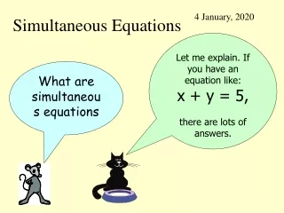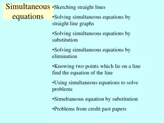
Simultaneous Equations
Simultaneous Equations. Lecture 22. Today’s plan. Simultaneous equation models Stating the problem How to estimate given simultaneity Instrumental variables and two stage least squares (TSLS). Example. L22.xls : examining the relationship between price and quantity

Simultaneous Equations
E N D
Presentation Transcript
Simultaneous Equations Lecture 22
Today’s plan • Simultaneous equation models • Stating the problem • How to estimate given simultaneity • Instrumental variables and two stage least squares (TSLS)
Example • L22.xls : examining the relationship between price and quantity • Two variables: hours and wages • Can construct a graph of labor demand and supply LS W We want to identify the relationship between hours and wages for workers LD H
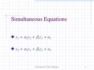
Structural model • In terms of labor demand and labor supply: (D): Hi = a1 + b1Wi + ui (S): Hi = a2 +b2Wi + c2Xi + d2NKi +vi where Xi = age and NKi = number of kids • Today we’ll estimate the labor supply curve for married women in California in 1980
Structural model (2) • We’ll assumelabor market equilibrium, or HiD = HiS • We’ll also assume that hours and wages are endogenous • Both are determined at the same time: either could be placed as the dependent variable for the model • Since hours and wages are determined simultaneously, there will be a relationship between wages and the error term ui
Reduced forms • Assuming labor market equilibrium a1 + b1Wi + ui = a2 + b2Wi + c2Xi + d2NKi + vi • Working with the equation, we have: • This gives us an expression for wages in terms of the exogenous variables • Here, our exogenous variables are: Xi, age, and NKi
Reduced forms (2) • We can rewrite the expression for wages in a simpler form: • This is the reduced form for wages • We can also get a reduced form for hours: • Original expression: Hi = a1 + b1Wi +ui • By rewriting it and substituting into the labor supply equation, we arrive at:
Reduced forms (3) • The reduced forms give the relationship between each of the endogenous variables and the exogenous variables • also show how the errors are related • Looking back at the derivation of the reduced form equations • see that each is composed of the error terms from both the labor demand and labor supply equation ui and vi
Reduced forms (4) • Errors from both the labor demand and labor supply curves show up in both of the reduced form equations: W LS vi ui LD H
Reduced forms (5) • If faced with the problem of simultaneity • model can be restated in terms of reduced forms • endogenous variables can be expressed solely in terms of exogenous variables • can estimate reduced forms using OLS if we have strictly exogenous variables on the right-hand-side • cannot recover structural parameters from the reduced form estimation • reduced forms only give an indication of the correlation between the endogenous and exogenous variables
Reduced forms (6) • Our example: can only get estimates of the effects of age and the number of kids on hours of work and wages separately • Three problems with reduced form estimation: • Xi and NKi are assumed to be exogenous - might not be true • Structural model isn’t estimated • Need structural model to examine more complex matters (example: effect of a tax cut on hours worked)
Instrumental variables and TSLS • Since we think wages and hours are simultaneously determined, we expect: • To estimate the model we will use instrumental variables, or two stage least squares (TSLS) • Our model is: Hi = a1 + b1Wi +ui • we need a proxy for Wiin order to get an unbiased estimate b1
Instrumental variables and TSLS (2) • Why we need a proxy • Assuming wages and hours are correlated, the errors on Hi will be correlated with Wi • if we can find a proxy for Wi that is correlated with Wi but not with the errors on Hi, we can get a consistent estimate of b1 • Our proxy will be an instrumental variable
Instrumental variables and TSLS (3) • We already know from the reduced form that wages are partially dependent on age and number of kids: Wi = 10 + 11Xi + 12NKi + 1i • What is a good proxy that’s independent of the endogenous variable? • Predicted wages because by construction, it has the errors taken out:
Instrumental variables and TSLS (4) • We can substitute in the predicted wage term into the expression for hours: • the predicted wage term is related to Wi and independent from the ui by construction • This is called two stage least squares
Two stage least squares • First stage: use OLS to estimate reduced form for the right-hand side endogenous variable Wi: Wi = 10 + 11Xi + 12NKi + 1i • Second stage: use predictions from the first stage for : • Then we estimate this model using the proxy for wages
Two stage least squares (2) • Why should TSLS work? • We have a set of exogenous, predetermined variables • The more exogenous variables we have, the better we can determine the endogenous variable of interest • Can test for over-identification (how many extra variables you have) using the Hausman test
Good empirical practice 1) Look at the reduced forms 2) Report the OLS results for the structural model (Hi = a1 + b1Wi + ui) • Since E(Wi, ui) 0, the OLS estimate for b1 will be biased 3) Report the two stage least squares results • consistent estimate with instrumental variables • inefficient because standard errors on coefficient of interest are inflated
Example • L22.xls : sample of married women in CA in 1980 • information on hours of work, age, wages, and number of kids • What do we notice? • The b1 is much larger & standard error on b1 is larger • Using instrumental variables: consistent but inefficient estimate • Consistent: no correlation between proxy variable and error • Still no clear relationship between predicted wages and hours of work! • Variance has increased