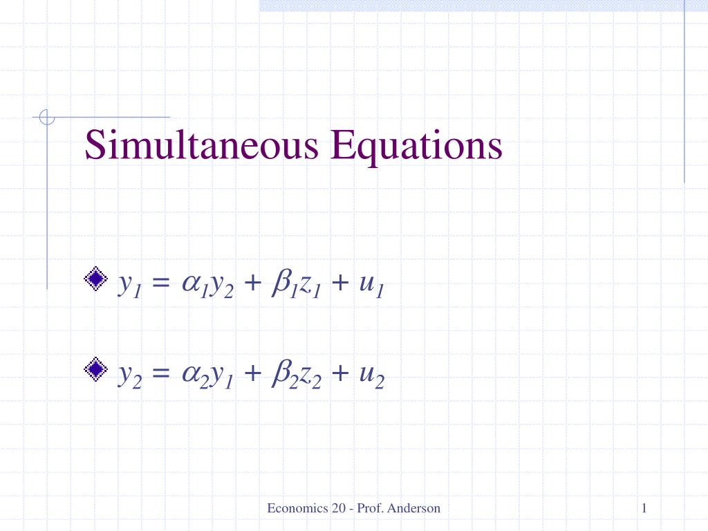
1. Simultaneous Equations y1 = a1y2 + b1z1 + u1 y2 = a2y1 + b2z2 + u2 Economics 20 - Prof. Anderson

2. Simultaneity • Simultaneity is a specific type of endogeneity problem in which the explanatory variable is jointly determined with the dependent variable • As with other types of endogeneity, IV estimation can solve the problem • Some special issues to consider with simultaneous equations models (SEM) Economics 20 - Prof. Anderson

3. Supply and Demand Example • Start with an equation you’d like to estimate, say a labor supply function • hs = a1w + b1z + u1, where • w is the wage and z is a supply shifter • Call this a structural equation – it’s derived from economic theory and has a causal interpretation where w directly affects hs Economics 20 - Prof. Anderson

4. Example (cont) • Problem that can’t just regress observed hours on wage, since observed hours are determined by the equilibrium of supply and demand • Consider a second structural equation, in this case the labor demand function • hd = a2w + u2 • So hours are determined by a SEM Economics 20 - Prof. Anderson

5. Example (cont) • Both h and w are endogenous because they are both determined by the equilibrium of supply and demand • z is exogenous, and it’s the availability of this exogenous supply shifter that allows us to identify the structural demand equation • With no observed demand shifters, supply is not identified and cannot be estimated Economics 20 - Prof. Anderson

6. Identification of Demand Equation S (z=z1) D w S (z=z2) S (z=z3) h Economics 20 - Prof. Anderson

7. Using IV to Estimate Demand • So, we can estimate the structural demand equation, using z as an instrument for w • First stage equation is w = p0 + p1z + v2 • Second stage equation is h = a2ŵ + u2 • Thus, 2SLS provides a consistent estimator of a2, the slope of the demand curve • We cannot estimate a1, the slope of the supply curve Economics 20 - Prof. Anderson

8. The General SEM • Suppose you want to estimate the structural equation: y1 = a1y2 + b1z1 + u1 • where, y2 = a2y1 + b2z2 + u2 • Thus, y2 = a2(a1y2 + b1z1 + u1) + b2z2 + u2 • So, (1 – a2a1)y2 = a2b1z1 + b2z2 + a2 u1 + u2, which can be rewritten as • y2 = p1z1 + p2z2 + v2 Economics 20 - Prof. Anderson

9. The General SEM (continued) • By substituting this reduced form in for y2, we can see that since v2 is a linear function of u1, y2 is correlated with the error term and a1 is biased – call it simultaneity bias • The sign of the bias is complicated, but can use the simple regression as a rule of thumb • In the simple regression case, the bias is the same sign as a2/(1 – a2a1) Economics 20 - Prof. Anderson

10. Identification of General SEM • Let z1 be all the exogenous variables in the first equation, and z2 be all the exogenous variables in the second equation • It’s okay for there to be overlap in z1 and z2 • To identify equation 1, there must be some variables in z2 that are not in z1 • To identify equation 2, there must be some variables in z1 that are not in z2 Economics 20 - Prof. Anderson

11. Rank and Order Conditions • We refer to this as the rank condition • Note that the exogenous variable excluded from the first equation must have a non-zero coefficient in the second equation for the rank condition to hold • Note that the order condition clearly holds if the rank condition does – there will be an exogenous variable for the endogenous one Economics 20 - Prof. Anderson

12. Estimation of the General SEM • Estimation of SEM is straightforward • The instruments for 2SLS are the exogenous variables from both equations • Can extend the idea to systems with more than 2 equations • For a given identified equation, the instruments are all of the exogenous variables in the whole system Economics 20 - Prof. Anderson