Spatial Analysis
Spatial Analysis. Longley et al., Ch 14,15. Transformations . Buffering (Point, Line, Area) Point-in-polygon Polygon Overlay Spatial Interpolation Theissen polygons Inverse-distance weighting Kriging Density estimation. Basic Approach. Map. New map. Transformation. Point-in-polygon.

Spatial Analysis
E N D
Presentation Transcript
Spatial Analysis Longley et al., Ch 14,15
Transformations • Buffering (Point, Line, Area) • Point-in-polygon • Polygon Overlay • Spatial Interpolation • Theissen polygons • Inverse-distance weighting • Kriging • Density estimation
Basic Approach Map New map Transformation
Point-in-polygon Select point known to be outside Select point to be tested Create line segment Intersect with all boundary segments Count intersections EVEN=OUTSIDE ODD=INSIDE
Combining maps • RASTER • As long as maps have same extent, resolution, etc, overlay is direct (pixel-to-pixel) • Otherwise, needs interpolation • Use map algebra (Tomlin) • Tomlin’s operators • Focal, Local, Zonal
Combining Maps • VECTOR • A problem
Creating new zones Town buffer River buffer
Other spatial analysis methods • Centrographic analysis (mean center) • Dispersion measures (stand. Dist) • Point clustering measures (NNS) • Moran’s I: Spatial autocorrelation (Clustering of neighboring values) • Fragmentation and fractional dimension • Spatial optimization • Point • Route • Spatial interpolation
Moran’s I http://gis.esri.com/library/userconf/proc02/pap1064/p106413.gif
Spatial autocorrelation • Correlation of a field with itself Low High Maximum
Spatial optimization www.giscenter.net/eng/work_03_e.html
Linear interpolation C B Half way from A to B, Value is (A + B) / 2 A
Nonlinear Interpolation • When things aren't or shouldn’t be so simple • Values computed by piecewise “moving window” • Basic types:1. Trend surface analysis / Polynomial 2. Minimum Curvature Spline 3. Inverse Distance Weighted 4. Kriging
1. Trend Surface/Polynomial • point-based • Fits a polynomial to input points • When calculating function that will describe surface, uses least-square regression fit • approximate interpolator • Resulting surface doesn’t pass through all data points • global trend in data, varying slowly overlain by local but rapid fluctuations
1. Trend Surface cont. • flat but TILTED plane to fit data • surface is approximated by linear equation (polynomial degree 1) • z = a + bx + cy • tilted but WARPED plane to fit data • surface is approximated by quadratic equation (polynomial degree 2) • z = a + bx + cy + dx2 + exy + fy2
2. Minimum Curvature Splines • Fits a minimum-curvature surface through input points • Like bending a sheet of rubber to pass through points • While minimizing curvature of that sheet • repeatedly applies a smoothing equation (piecewise polynomial) to the surface • Resulting surface passes through all points • best for gently varying surfaces, not for rugged ones (can overshoot data values)
3. Inverse Distance Weighted • Each input point has local influence that diminishes with distance • estimates are averages of values at n known points within window R where w is some function of distance (e.g., w = 1/dk)
IDW • IDW is popular, easy, but problematic • Interpolated values limited by the range of the data • No interpolated value will be outside the observed range of z values • How many points should be included in the averaging? • What about irregularly distributed points? • What about the map edges?
IDW Example • ozone concentrations at CA measurement stations 1. estimate a complete field, make a map 2. estimate ozone concentrations at specific locations (e.g., Los Angeles)
Ozone in S. Cal: Text Example measuring stations and concentrations (point shapefile) CA cities (point shapefile) CA outline (polygon shapefile) DEM (raster)
Power of distance 4 sectors Further define interpolation method
Cross validation • removing one of the n observation points and using the remaining n-1 points to predict its value. • Error = observed - predicted
4. Kriging • Assumes distance or direction betw. sample points shows a spatial correlation that help describe the surface • Fits function to • Specified number of points OR • All points within a window of specified radius • Based on an analysis of the data, then an application of the results of this analysis to interpolation • Most appropriate when you already know about spatially correlated distance or directional bias in data • Involves several steps • Exploratory statistical analysis of data • Variogram modeling • Creating the surface based on variogram
Kriging • Breaks up topography into 3 elements:Drift (general trend), small deviations from the drift and random noise. To be stepped over
Explore with Trend analysis • You may wish to remove a trend from the dataset before using kriging. The Trend Analysis tool can help identify global trends in the input dataset.
Kriging Results • Once the variogram has been developed, it is used to estimate distance weights for interpolation • Computationally very intensive w/ lots of data points • Estimation of the variogram complex • No one method is absolute best • Results never absolute, assumptions about distance, directional bias
Kriging Example Surface has no constant mean Maybe no underlying trend surface has a constant mean, no underlying trend allows for a trend binary data
Kriging Result • similar pattern to IDW • less detail in remote areas • smooth
IDW vs. Kriging • Kriging appears to give a more “smooth” look to the data • Kriging avoids the “bulls eye” effect • Kriging gives us a standard error Kriging IDW