Download
1 / 38
380 likes | 402 Vues
Explore revealed and stated preference methods, hedonic pricing, regression modeling, and valuation of life in cost-benefit analysis. Learn to assess the value of environmental amenities and human life.

E N D
Benefit-Cost Analysis: Measuring Benefits, pt II
Roadmap progress…. • A. Stated preference • Contingent valuation • Choice modeling • B. Revealed preference • Hedonic pricing (prices, wages) • Property value • Wage rates • Travel cost • Defensive behavior • Cost of illness (COI) • Materials damage (maintenance, repair, replacement)
B. Revealed Preference • Depends on a relationship between a market and non-market good. • Behavior trail • Estimate the market “footprint” of non-market goods (bads) (Russell 2001) • For use value only
Revealed Pref: Hedonic Pricing Methods • Idea: if the price of something is related to multiple characteristics, look at the differences in prices to assess value buyers place on one of those characteristics. • Key concept -- Bundled goods: People value goods based on a bundle of attributes. (Couling, 2001) For overview see Taylor (Chp 10) in Champ et al. (2003)
“Regression” is a method for estimating the relationship between things. Eg: how does nearby water quality affect home prices? home price ($) Estimated model observed data water quality index ( better) (Relinad Youngblood, NC State U.)
“Multiple regression” allows for >1 variable to have influence. Eg: how do (1) nearby water quality, and (2) lot size affect home prices? home price ($) Estimated model observed data water quality index ( better) lot size (Source: Relinad Youngblood, NC State U.)
Hedonic Property Pricing Model Approach: statistically break down the value of a good into its component parts to isolate the value of the environmental attribute. (Aside: This equation is linear but nonlinear forms are common--see Taylor 2003) • P: housing price • H: structural and property characteristics • bedrooms, lot size, … • N: neighborhood characteristics • median income, school quality, …. • L: location characteristics • level of the environmental amenity • ε: error term for unobservables MWTP for the env. amenity Can use to evaluate amenities and/or disamenities Bruegel: The Triumph of Death
Hedonic Property Value Example nothin' SUP? Leggett and Bockstael (2000) • Estimate the value of water quality in Chesapeake Bay • Water quality: reported faecal coliform levels (affects utility from recreational use) • Result: 1 unit (count/ml) increase in median annual concentration of pollution property value falls by $5,000.
Hedonic wage method is used to estimate value of increased risk of on-the-job mortality to use as the “value of a statistical life” (VSL). • Wage rates higher for those willing to accept riskier jobs (all else =). • Idea: Wage differential between two jobs differing only in risk of death provides an implicit VSL • Valuation of occupational risk, applied to environmental risk (benefits transfer) US Bureau of Labor Stat. (2014) Logging worker mortality: 109.5/100K > 33 times that of the average U.S. worker (3.3/100K
Estimating benefits of reducing deaths • For a risk not currently incurred: • VSL = Δwealth / Δp = $WTA/ Δp here WTA is willingness-to-accept increased risk Eg: individuals demand $4 to accept an increase the risk of death of 2x10⁻⁶ Thus: • $WTA = $4, Δp=2x10⁻⁶. VSL = $WTA/ Δp = $4 / (2x10⁻⁶) = $2M
The VSL is not intended to reflect the intrinsic value of a life • Rather: convenient, imperfect, one-size-fits-all measure of individuals’ demand for risk reductions in small units. • Its estimation and its use are usually in units of 10-6 (changes in the probability of death in the “millionths”) • A VSL of $7M implies that an individual would be willing to pay $7.00 to reduce their risk of death by 10-6 • If a policy reduced the mortality risk of everyone in the U.S. by 10-6, then with a VSL of $7M (or $7 x 10⁶), the benefit could be estimated by: • (VSL x Δp ) x (number affected) • ([$7x106] x 10-6 ) x (3x10⁸ ) • $7 x 3x108 = $2.1B • (VSL ) x (Δp x number affected) • ($7x106) x (10-6 x 3x108 ) • $7x106 x 300 = $2.1B $7 benefit/person times number of people 300 “expected lives saved” times VSL
EPA: What Does it Mean to Place a value on life? • “The EPA does not place a dollar value on life,… • but [we do] try to estimate the benefits from reducing the risk of death from environmental contaminants. … • How do people value, in dollar terms, this small (but important) reduction to their risk of dying? • The process of valuing risk [aka the process of valuing "statistical life“] does not produce an estimate of the value of life itself.“ What is the "Value of a Statistical Life"? • the aggregate estimated value of reducing small risks across a large number of people. • based on how people themselves would value reducing these risks. Source: http://yosemite1.epa.gov/ee/epa/eed.nsf/pages/MortalityRiskValuation.htm
Pop quiz • The average annual workplace mortality rate in the U.S. is approximately 4/100,000. • The average worker earns about $45,000 per year. • Suppose we ignore all other job attributes and observe on average that workers demand a salary of at least $45,050 a year to accept jobs that have a 5/100,000 mortality rate. • What is the implied value of a statistical life? (Make sure to write out the expression used to generate the number.)
Revealed Preference: Travel cost • Estimate value of an amenity (e.g. park) by treating the costs incurred to experience it as its “price”. • Idea: travel and the recreational area are complements (consumed together) • Information needs (gathered via survey): • # of trips taken (by indiv’ls/households) to a particular site in a year • their travel cost to that site • Monetary (out-of-pocket cost: gas, hotel, etc) • Opportunity cost of leisure time (shadow value of time constraint, e.g. 1/3 to 1/2 wage rate)
Travel cost example • Focus on the behavior of the Worthingtons, a single family who lives a given distance away from a free public park. • Survey work Worthingtons visits this park an average of four days/year. • Estimate their travel costs to go from their home to the park and return. • cash travel cost (gas, wear and tear on the car, food, etc.) is $18 per trip • round trip takes one hour each way (need to put a value on the time spent traveling) • tricky: need value foregone, in terms of salary or other income, by spending this time traveling rather than working. • Empirical work ⅓ to ½ of the wage rate; • assume their travel time is worth $8.00 per hour Roundtrip cost of travel time: $8 * 2 = $16 • Price the Worthingtons “pay” for each visit to the park is the total cost of the trip: $18 + $16 = $34.
Travel cost example: Calculating the value • Suppose: there are only three other families within range of the park • Surveyed travel costs for all four: Assume: • each family is identical except for their travel cost (can treat the table as any individual family’s demand schedule) • demand is linear (a straight line). (Worthingtons) • Calculate (chalkboard exercise—review of plotting demand curve, calc. of benefits, consumer surplus) • For each individual in this “world” calculate • (Gross) benefit (B) of the park (given their observed number of visits) • Net benefit of the park (recall NB = B-C) • Then sum these values to find the aggregate (1) benefit, and (2) net benefit of the park. • Have we estimated the complete value of the park to these families? What component of the complete value have we estimated? Use value or non-use value? Was this stated or revealed preference?
Pop quiz You are asked to interpret the results of a travel cost survey. The figure presents data for two families (1 and 2), including their travel cost per trip (p) and the number of trips they take (q). Assume that the families are identical except for their travel costs. The figure also presents a marginal willingness to pay (demand) curve (assuming that a straight line between points). • Explain what is represented by area “a” in the figure (1 sentence): • Explain what is represented by area “a + b” in the figure (1 sentence): • Suppose the price of hotels at the park rose significantly for these families (but all other attributes remained the same). What change in behavior of the families would we predict? What would be the implications for the quantities you discussed in part A and B above? (2 sentences).
Travel cost caveats • in practice much more complicated • Families will differ in terms of many factors (not just in travel costs) • income levels, presence of alternative parks and other recreational experiences available to them, etc. • Solution: collect large amounts of data on many visitors; statistically sort out various influences on park visitation rates.
Revealed Preference Methods Adapted from Boyle (Chp 8 in Champ et al. 2003)
Arsenic Hells Canyon Exxon Valdez VSL Chesap. Bay Pearce et al. (2006, Chp. 6)
Revealed versus stated pref. Econometrics lab, UCB (http://elsa.berkeley.edu/eml/qca_reader/9.combin.pdf)
Hells Canyon travel cost example: you don’t need perfect information to inform decisions The Situation • Hells Canyon on the Snake River (separating Oregon and Idaho) • spectacular vistas, outdoor amenities, important fish and wildlife habitat • economic potential as a site to develop hydropower • Generating hydropower damlarge lakesignificantly and permanently alter the ecological and aesthetic characteristics of Hell Canyon. The BCA Challenge • 1970’s: Env. economists from Resources For The Future in Washington, D.C. • asked to develop an economic analysis to justify preserving Hell Canyon in its natural state http://www.fs.fed.us/hellscanyon/ *Example from: http://www.ecosystemvaluation.org/travel_costs.htm http://upload.wikimedia.org/wikipedia/commons/3/36/OR_hells_canyon.jpg
Hells Canyon travel cost example: you don’t need perfect information to inform decisions The Analysis • Economic value of project: Net economic value (cost savings) of producing hydropower at Hells Canyon was $80,000 higher than at the "next best" site which was not environmentally sensitive. • Task: Estimate the economic value of losing the environmental amenities of Hells Canyon: Travel cost survey valuation: $900,000 • TCS was low-cost/low precision • But researchers did not attempt to strongly defend the "scientific" credibility of the valuation method/results. • Emphasized that, even if the "true value" of recreation at Hell Canyon was ten times less (i.e. $90k), it would still be greater than economic payoff from generating power there ($80k). The Results • Based largely on the results of this non-market valuation study, Congress voted to prohibit further development of Hell Canyon.
Benefits transfer takes valuation results from one setting and applies them in an alternative setting. 2. using estimates from pre-existing, “primary studies” “primary valuation” (Image source: Conservation Strategy Fund, 2016) 1. value a change in the “policy case” Benefits transfer: cheaper, faster, less accurate 3. adjust for differences charac-teristics that affect demand (WTP)
Kopp et al. 1997
Hedonic property value method • Potentially suited for valuing: noise abatement, proximity to waste sites or open space, air pollution, water quality. • Since no market exists for the amenity “peace and quiet”, we have no direct market evidence on how much this amenity is valued where people live. But, it can be traded implicitly in the property market. (Pearce 2006, chp 7). • Issues • Based on marginal changes: Appropriate to estimate small changes in environmental quality (large changes can lead to a change in the hedonic price function due to renegotiation from buyers and sellers as the supply of env. quality shifts) • Large data requirements (potential for omitted variable bias) • multicollinearity: nonmarket characteristics tend to move in tandem (e.g. properties near to roads have greater noise pollution and higher concentrations of air pollutants) • difficult to “tease out” the independent effect of these two forms of pollution
2016 Source: Margaret Cronin Fisk (Bloomberg) 1/8/16
Discussion question • Should government agencies use VSL estimates for valuation of public policies that reduce the risk of premature mortality? • Ackerman and Heinzerling (2004) • "In this approach [of assigning dollar values to human life, human health, and nature itself] formal cost-benefit analysis often hurts more than it helps: it muddies rather than clarifies fundamental clashes about values. … • [E]conomic theory gives us opaque & technical reasons to do the …wrong thing." • Sunstein (2004): • “(W)henever government decides how much to reduce risks, it is implicitly assigning such values. … Any regulator will acknowledge that at some point the cost of additional risk reduction is just too high. Why not be honest about that? • …the current system of regulation [shows] unjustified patterns -- large sums devoted to small risks, small sums devoted to large risks. The government's decisions will be far more transparent [and] consistent, if the government says how much it is willing to pay to prevent a risk of death. “
General issues with hedonic methods • Models generally assume that households/individuals have perfect information about attributes of the property/job. • Simultaneity: causality • Property: causality between env. quality and price (e.g. higher quality leads to higher price, larger tax base, more money for env. quality). • Wage: causality between risk and wages can go both ways (e.g. higher wage to compensate for air pollution but high wage attracts more workers leading to change in air quality)
Revealed Preference: Travel cost • Trace out the MWTP curve (or demand curve) for a particular amenity, like a national park. • v: trips • cv: trip cost to given site • cs: trip cost to alternative site(s) • y: income • z: demographic variables $ f(cv, cs, y, z) A cv0 B • A+B: total WTP for trips • B: total trip cost • A: “access value”, total consumer surplus for trips to site in year. v0 trips, v Access value: linear single-site model Parsons (Chp 9 in Pearce et al. 2006)
Travel cost example: South African game reserves (Day, 2002) • What would be the lost welfare to domestic visitors to four game parks? • Data: survey of 1,000 visitors • Demonstrates the effect of site substitutes. “Mr. Shuffles” TorstenBlackwood/AFP/Getty Images.
Revealed Preference: Defensive Behavior --> • Estimate willingness to pay to reduce a “bad” by looking at avoidance expenditures made to reduce the risk or the impact of the bad. When faced with water of dubious quality how much do individuals spend to improve their drinking water (expenditures: filters and bottled water) 2015
Revealed Pref: Cost of illness • Used to estimate benefits from policies which result in increased health • Easy to understand • Not grounded in consumer choice and welfare theory (in contrast to other methods) • No estimate of marginal pricing or surplus