Understanding Homogeneous Coordinates in 2D and 3D Surface Modelling
This lecture covers the essentials of modeling with homogeneous coordinates in 2D and 3D, emphasizing their significance in translating points and creating rational curves such as Bézier and B-spline curves. It explains how points at infinity cannot be projected onto a plane and the relationship between control points and curve shaping. The discussion extends to surfaces generated from these curves, focusing on continuity properties and adaptive subdivision methods for rendering Bézier surfaces. This intricately ties together the relationships between control points, curves, and surfaces in computer graphics.

Understanding Homogeneous Coordinates in 2D and 3D Surface Modelling
E N D
Presentation Transcript
Surfaces Lecture 6 (Modelling)
Reminder: Homogenous Co-ordinates • 2D Translations cannot be encoded using matrix multiplication because points at the origin never move. • Instead use homogenous co- ordinates • These are projections of 3D points along a ray from the origin onto the plane .
Homogenous Projections • An infinite number of homogenous co-ordinates map to every 2D point. are all equivalent to . • Points at infinity have and cannot be projected onto the plane because this would involve division by zero. • Conversion: • All of the above also applies to 3D homogenous co-ordinates:
Matrices for Homogenous Co-ordinates where is a standard transformation. • Translation:
Rational Curves • The control points of a Bézier or B-spline curve can be encoded in homogenous co-ordinates: • Rational curves have the form: • NURBS (Non-Uniform Rational B-spline) curves are the homogenous version of standard B-spline curves.
Behaviour of Rational Curves • The fourth co-ordinate provides additional control and acts as a weighting term. • If then behaves as normal then attracts the curve then repulses the curve is disallowed because it contravenes the convex hull property. • Strictly speaking, the behaviour of weighted control points is relative, rather than absolute. If all are set at then this enforces the same behaviour as all . • Rational curves have two advantages: • They provide further control over the shape of the curve. • They can exactly represent conic sections (e.g. a circle). • BUT they are more computationally costly.
Exercise: Knot Vectors and B-splines • Determine the number of curve segments, number of spans ( ), curve domain, and continuity at the knots for the B-spline curves with the following knot vectors: (a) (b) • Given the control points below (corresponding to these knot vectors) establish convex hulls and draw a rough sketch of the curves in each case: (a) (b)
Solution I: Knot Vectors and B-splines • (a) curve segments and . At knot the multiplicity is and continuity is . This is a discontinuity in position (a jump). (b) curve segments and . The curve interpolates and . At knot the multiplicity is and continuity is . • (a) (b)
Surfaces • Curves generalise to Surfaces: • A surface is a function of two variables rather than just one . • A rectangular surface has a curve running along each of its four edges. • A rectangular surface can be envisioned as a curve which changes its shape as it is swept through space. Each control point of the initial curve is moved along a path which is itself a curve. • Surface Definition: • An -degree by -degree Bézier patch is defined by control points :
Surface Properties • Adjacent control points can be connected to form a control net (which serves the same purpose as a control polygon). • The degrees along and do not have to match. • B-spline surfaces are a similar extension of B-spline curves. • Continuity between patches: • C0: continuous in position. The four edge c.p. must match. • C1: continuous in position and tangent vector. The two control points on either side of each edge c.p. must be colinear with the edge point and each other and be equidistant from the edge point. • Algorithms (e.g. de Casteljau subdivision) and properties (e.g. convex hull) still apply with some small modification.
Example Surface • Example: cubic Bézier patch • The four corner c.p. are interpolated. • Each edge is a curve defined by four c.p. • There are four interior c.p. determining the inner shape.
Rendering Bézier Surfaces • Adaptive Subdivision: Use a collection of planar polygons to approximate the surface. • Check if a quadrilateral with corners at the endpoints is an adequate approximation to the surface. • If so, halt recursion. • If not, subdivide into two smaller Bézier patches using bi-parametric de Casteljau. Subdivision must alternate in and on successive recursive subdivisions. • Need to specify a tolerance for when the quadrilateral is an adequate approximation. • The set of resulting (non-planar) quadrilaterals is further subdivided into (planar) triangles. • A B-Spline surface can be converted to a set of Bézier patches by a process of knot insertion and then rendered.
Subdivision Surfaces • Motivation: • Creating objects from Bézier or B-spline patches is very difficult if they have a non-planar topology. For instance a C1 sphere cannot be constructed from non-degenerate patches. • Complex topologies with many-sided patches are possible if a subdivision approach is adopted. • Method: • Similar to Chaikin’s corner cutting. • Start with a closed control net (which roughly approximates the shape of the object). • Successively refine the control net by introducing new control points. In the limit this produces a smooth surface. • Proviso: • The surface may have exception points where it is not as smooth.
Doo-Sabin Subdivision • Mostly produces a quadratic B-spline surface. • Algorithm: • Input: an arbitrary open or closed polyhedron. • Output: a smooth surface. • Refinement: • (1) Find the centroid of each face (average its vertices). • (2) Find the midpoints of all straight lines connecting the centroid to its defining vertices. • (3) Construct a new polyhedron from these midpoints by forming: • E-faces. For a given edge there are four midpoints controlled by its endpoints. Connect these midpoints into a rectangle. • V-faces. Form a face with the midpoints that surround an original vertex. • F-faces. Connect the midpoints belonging to the same face.
Geri’s Game: Subdivision Surfaces • Subdivision Surface Technology: • Sharp creases created by delaying subdivision of an edge (wrinkles). • Clothing simulation by efficient collision detection between subdivision surfaces (jacket). • Constructing smooth scalar fields on subdivision surfaces for shading and texturing (skin). • Source: • De Rose, T., Kass, M. and Teoung, T. “Subdivision Surfaces in Character Animation”, SIGGRAPH ’98, pp. 85-94.
Bézier Triangles: Barycentric Co-ords • The location of a point within a triangle can be expressed in barycentric co-ordinates. • Even though there are three parameters this is still a surface because they are not independent. Depends on and .
Bézier Triangles: Notation • A degree Bézier triangle has control points. • Each control point is labelled by three values with the condition that . • Corner CP have or or and the other indices . • A point on the Bézier triangle at Barycentric co-ordinates has the Bernstein form:
Bézier Triangles: Control Points • Linear: • Quadratic: • Cubic:
Bézier Triangles: de Casteljau Algorithm • Abbreviations: • Algorithm: • Given a triangular array of CP and barycentric co-ordinates : • where and and is the point at on the Bézier triangle.