Surfaces
Surfaces. Chiew-Lan Tai. Reading. Required Hills Section 11.11 Hearn & Baker, sections 8.11, 8.13 Recommended Sections 2.1.4, 3.4-3.5, 3D Computer Graphics, Watt. Mathematical surface representations. Explicit z = f(x,y) (a.k.a. “height field”)

Surfaces
E N D
Presentation Transcript
Surfaces Chiew-Lan Tai
Reading Required • Hills Section 11.11 • Hearn & Baker, sections 8.11, 8.13 Recommended • Sections 2.1.4, 3.4-3.5, 3D Computer Graphics, Watt
Mathematical surface representations • Explicit z = f(x,y) (a.k.a. “height field”) What if the surface isn’t a function? • Implicit g(x,y,z) = 0 x2 + y2 + z2 = 1 • Parametric S(u,v) = (x(u,v), y(u,v), z(u,v)) x(u,v) = r cos 2v sinu y(u,v) = r sin 2v sinu z(u,v) = r cos u 0≤u≤1, 0≤v≤1
Tensor product Bézier surfaces • Given a grid of control point Vij, forming a control net, construct a surface S(u,v) by: • Each row in u-direction is control points of a curve Vi(u). • V0(u), …, Vn(u) at a specific u are the control points of a curve parameterized by v (i.e. S(u,.v))
Tensor product Bezier surfaces, cont. • Let’s walk through the steps: • Which control points are interpolated by the surface? Only the 4 corner points
Tensor product Bezier surfaces, cont. • Writing it out explicitly: • Linear Bezier surface: • Quadratic Bezier surface?
Matrix form • For the case of cubic Bezier surface:
Tensor product B-spline surfaces • Like spline curves, we can piece together a sequence of Bezier surfaces to make a spline surface. If we enforce C2 continuity and local control, we get B-spline curves:
Tensor product B-spline surfaces • Use each row of B control points in u to generate Bezier control points in u. • Treat each row of Bezier control points in v direction as B-spline control points to generate Bezier control points in v direction. u
Surface normal S S S S
Rotational surfaces (surface of revolution) • Rotate a 2D profile curve about an axis
Constructing surfaces of revolution • Given a curve C(u) in the yz-plane: • Let Ry() be a rotation about the y-axis • Find: A surface S(u,v) obtained by applying Ry() on C(u) S(u,v) = Ry(v) [0, Cy(u), Cz(u), 1]t y Profile curve, C(u) z x
Surface of revolution y • Profile curve on yz plane: C(u) = ( 0, Cy(u), Cz(u) ) • The surface S(u,v) obtained by rotating C(u) about the y-axis is S(u,v) = ( -Cz(u) sin(v), Cy(u), Cz(u) cos(v)) x z
General sweep surface • Given a planar profile curve C(u) and a general space curve T(v) as the trajectory, sweep C(u) along the trajectory • How to orient C(u) as it moves along T(v)?
Orientating C(u) • Define a local coordinate frame at any point along the trajectory • The Frenet frame (t,n,b) is the natural choice • As we move along T(v), the Frenet frame (t,b,n) varies smoothly (inflection points where curvature goes to zero needs special treatment)
Sweep Surfaces • Orient the profile curve C(u) using the Frenet frame of the trajectory T(v): • Put C(u) in the normal plane. • Place Oc at T(v). • Align xc of C(u) with b. • Align yc of C(u) with n. • Sweep surface S(u,v) = T(v) + n(v)Cx(u) + b(v) Cy(u)
Variations • Several variations are possible: • Scale C(u) as it moves, possibly using length of T(v) as a scale factor. • Morph C(u) into some other curve C’(u) as it moves along T(v)
Summary What to take home: • How to construct tensor product Bezier surfaces • How to construct tensor product B-spline surfaces • How to construct surfaces of revolution • How to construct sweep surfaces from a profile and a trajectory curve with a Frenet frame
Subdivision Surfaces What’s wrong with B-spline/NURBS surfaces?
Subdivision curves Idea: • repeatedly refine the control polygon • curve is the limit of an infinite process.
Chaikin’s algorithm • In 1974, Chaikin introduced the following “corner-cutting” scheme: • Start with a piecewise linear curve • Repeat • Insert new vertices at the midpoints (the splitting step) • Average two neighboring vertices (the average step) Averaging mask (0.5, 0.5) • With this averaging mask, in the limit, the resulting curve is a quadratic B-spline curve.
Local subdivision mask • Subdivision mask: ¼ (1, 2, 1) • Splitting and averaging: • Applying the step recursively, each vertex converges to a specific point • With this mask, in the limit, the resulting curve is a cubic B-spline curve.
General subdivision process • After each split-average step, we are closer to the limit surface. • Can we push a vertex to its limit position without infinite subdivision? Yes! • We can determine the final position of a vertex by applying the evaluation mask. The evaluation mask for cubic B-spline is 1/6 (1,4, 1)
DLG interpolating scheme (1987) • Algorithm: • splitting step introduces midpoints, and averaging step only changes these midpoints • Dyn-Levin-Gregory scheme:
Building Complex Models • This simple idea can be extended to build subdivision surfaces.
Subdivision surfaces • Iteratively refine a control polyhedron (or control mesh) to produce the limit surface using splitting and averaging step: • There are two types of splitting schemes: • vertex schemes • face schemes
Vertex schemes • A vertex surrounded by n faces is split into n subvertices, one for each face: • Doo-Sabin subdivision:
Face schemes • Each quadrilateral face is split into four subfaces: • Catmull-Clark subdivision:
Face scheme, cont. • Each triangular face is split into four subfaces: • Loop subdivision:
Averaging step • Averaging masks:
Adding creases • Sometimes, a particular feature such as a crease should be preserved. • we just modify the subdivision mask. • This gives rise to G0 continuous surfaces.
Creases • Here’s an example using Catmull-Clark surfaces:
Object Deformation • Many objects are not rigid • jello, mud, gases, liquids • In animation, to give characterization to rigid objects • stretch and squash • Two main classes of techniques • Geometric-based • Physically-based
Geometric Deformations • Deform the object’s geometry directly • control point / vertex manipulation • Deform the object’s geometry indirectly • Warp the space in which the object is embedded (Spatial Deformation) • Main techniques • Nonlinear Deformation (Barr) • Free Form Deformation (FFD) • Curve-based Deformation
Spatial Deformation:General framework • Warps the space that the mesh is embedded in • User inputs pairs of features to guide the deformations • point pairs • local coordinate frames • continuous curves
Spatial Deformation:General framework • User inputs pairs of features to guide the deformations • discrete point pairs • local coordinate frames • Continuous curves
Spatial Deformation:General framework • Spatial deformation defines a mapping on the space that surrounds the model • It can be performed on any models that use point-based data • pixels in images • control points in spline surfaces • Vertices in mesh • point cloud data • Deformation is propagated along the space • May not be what the user expects
Freeform Deformation (FFD)[Sederberg and Parry 1986] • Define a volume using parallelepiped lattice • Lattice defines a coordinate system (S,T,U) • Modify the lattice points • Deformation of a point in the space depends on its (s,t,u) coordinates
Freeform Deformation (FFD) The lattice defines a Bezier volume: For each object point v, determine its lattice coordinates (s, t, u) Alter the lattice points New position of v is evaluated as P(s,t,u)
Axial Deformation [Lazarus 1994] Source curve R(u) target curve T(u) P P’ y’(u) Y(u) x’(u) T(u) R(u) x(u)
Wires”[Singh and Fiume 1998] • Defined curves “bound” on the surface • User deforms the mesh by editing the curves • The original and modified curves are feature pairs • Includes local rotation and scaling controls • Provide smooth composite deformation for multiple curve features