Riemann Sums
Riemann Sums. Approximating Area. One of the classical ways of thinking of an area under a curve is to graph the function and then approximate the area by drawing rectangular or trapezoidal regions under the curve (or nearly so). .

Riemann Sums
E N D
Presentation Transcript
Riemann Sums Approximating Area
One of the classical ways of thinking of an area under a curve is to graph the function and then approximate the area by drawing rectangular or trapezoidal regions under the curve (or nearly so).
Finding the area of each region is easy with rectangles, and these areas can be added to approximate the area of the function. f a b Here we approximate the area under f between a and b. Note that the rectangles do not all have the same width.
f a b This area is an approximation of
This method is one of several that can be used if we are unable to find an antiderivative of a function, and therefore cannot evaluate an integral symbolically, as we have been doing.
This methd can be used when an antiderivative can be found, but this is usually done for instructional purposes.
In order to approximate the area under the curve from 0 to 4, we can use a left sum with 2 subintervals. Note the way to write and calulate L2. The left sum uses the height at the left side of each subinterval.
Similarly we find a right sum with 2 subintervals. The right sum uses the height at the right side of the subinterval.
A midpoint sum uses the midpoint of each subinterval to define the height.
Finally, a trapezoidal sum uses the area of trapezoids instead of reactangles. These may be calculated from the function, or recognized as the average of L2 and R2.
If we increase the number of subintervals to 4 we can repeat the processes. The approximation will be better with smaller subintervals.
As the number of subintervals increase the approximation get closer to the true area under the curve. Usually, the calculations are not made by hand, but utilize software for this purpose.
You have probably noticed that sometimes you can predict whether a given sum will be an over or underestimate. Talk this over and see if you can come up with circumstances where you can predict over- or underestimates.
The heights are always determined by the value of the function, sometimes given in a table, sometimes found from a formula. This is a very brief overview and should be supplemented by reading Section 5.6 in your text.