Download
1 / 61
610 likes | 709 Vues
Analysis of data from the observation of an exotic S=+1 baryon in exclusive photoproduction from the deuteron, discussing statistical significance, Bayesian analysis, and hypothesis testing methods in particle physics discoveries. Includes a detailed examination of p-values, goodness-of-fit tests, and distinguishing true discoveries from statistical fluctuations to enhance data interpretation.

E N D
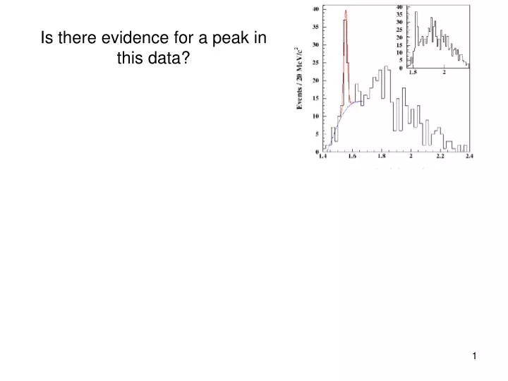
Is there evidence for a peak in this data? “Observation of an Exotic S=+1 Baryon in Exclusive Photoproduction from the Deuteron” S. Stepanyan et al, CLAS Collab, Phys.Rev.Lett. 91 (2003) 252001 “The statistical significance of the peak is 5.2 ± 0.6 σ”
Is there evidence for a peak in this data? “Observation of an Exotic S=+1 Baryon in Exclusive Photoproduction from the Deuteron” S. Stepanyan et al, CLAS Collab, Phys.Rev.Lett. 91 (2003) 252001 “The statistical significance of the peak is 5.2 ± 0.6 σ” “A Bayesian analysis of pentaquark signals from CLAS data” D. G. Ireland et al, CLAS Collab, Phys. Rev. Lett. 100, 052001 (2008) “The ln(RE) value for g2a (-0.408) indicates weak evidencein favour of the data model without a peak in thespectrum.” Comment on “Bayesian Analysis of Pentaquark Signals from CLAS Data” Bob Cousins, http://arxiv.org/abs/0807.1330
p-values and Discovery Louis Lyons IC and Oxford l.lyons@physics.ox.ac.uk TRIUMF, May 2012
TOPICS Discoveries H0 or H0 v H1 p-values: For Gaussian, Poisson and multi-variate data Goodness of Fit tests Why 5σ? Blind analyses What is p good for? Errors of 1st and 2nd kind What a p-value is not P(theory|data) ≠ P(data|theory) THE paradox Optimising for discovery and exclusion Incorporating nuisance parameters
DISCOVERIES “Recent” history: Charm SLAC, BNL 1974 Tau lepton SLAC 1977 Bottom FNAL 1977 W,Z CERN 1983 Top FNAL 1995 {Pentaquarks ~Everywhere 2002 } ? FNAL/CERN 2010? ? = Higgs, SUSY, q and l substructure, extra dimensions, free q/monopoles, technicolour, 4th generation, black holes,….. QUESTION: How to distinguish discoveries from fluctuations?
Penta-quarks? Hypothesis testing: New particle or statistical fluctuation?
H0 or H0 versus H1 ? H0 = null hypothesis e.g. Standard Model, with nothing new H1 = specific New Physics e.g. Higgs with MH = 120 GeV H0: “Goodness of Fit” e.g. χ2, p-values H0 v H1: “Hypothesis Testing” e.g. L-ratio Measures how much data favours one hypothesis wrt other H0 v H1 likely to be more sensitive or
Testing H0: Do we have an alternative in mind? 1) Data is number (of observed events) “H1” usually gives larger number (smaller number of events if looking for oscillations) 2) Data = distribution. Calculate χ2. Agreement between data and theory gives χ2 ~ndf Any deviations give large χ2 So test is independent of alternative? Counter-example: Cheating undergraduate 3) Data = number or distribution Use L-ratio as test statistic for calculating p-value 4) H0 = Standard Model
p-values Concept of pdf y Example: Gaussian μ x0 x y = probability density for measurement x y = 1/(√(2π)σ) exp{-0.5*(x-μ)2/σ2} p-value: probablity that x ≥ x0 Gives probability of “extreme” values of data ( in interesting direction) (x0-μ)/σ 1 2 3 4 5 p 16% 2.3% 0.13% 0. 003% 0.3*10-6 i.e. Small p = unexpected
p-values, contd Assumes: Gaussian pdf (no long tails) Data is unbiassed σ is correct If so, Gaussian x uniform p-distribution (Events at large x give small p) 0 p 1
p-values for non-Gaussian distributions e.g. Poisson counting experiment, bgd = b P(n) = e-b* bn/n! {P = probability, not prob density} b=2.9 P 0 n 10 For n=7, p = Prob( at least 7 events) = P(7) + P(8) + P(9) +…….. = 0.03
Poisson p-values n = integer, so p has discrete values So p distribution cannot be uniform Replace Prob{p≤p0} = p0, for continuous p by Prob{p≤p0} ≤ p0, for discrete p (equality for possible p0) p-values often converted into equivalent Gaussian σ e.g. 3*10-7 is “5σ” (one-sided Gaussian tail) Does NOT imply that pdf = Gaussian
Significance • Significance = ? • Potential Problems: • Uncertainty in B • Non-Gaussian behaviour of Poisson, especially in tail • Number of bins in histogram, no. of other histograms [FDR] • Choice of cuts (Blind analyses) • Choice of bins (……………….) • For future experiments: • Optimising could give S =0.1, B = 10-6
Goodness of Fit Tests Data = individual points, histogram, multi-dimensional, multi-channel χ2 and number of degrees of freedom Δχ2 (or lnL-ratio): Looking for a peak Unbinned Lmax? Kolmogorov-Smirnov Zech energy test Combining p-values Lots of different methods. Software available from: http://www.ge.infn.it/statisticaltoolkit
χ2 with ν degrees of freedom? • ν = data – free parameters ? Why asymptotic (apart from Poisson Gaussian) ? a) Fit flatish histogram with y = N {1 + 10-6 exp{-0.5(x-x0)2} x0 = free param b) Neutrino oscillations: almost degenerate parameters y ~ 1 – A sin2(1.27 Δm2 L/E) 2 parameters 1 – A (1.27 Δm2 L/E)2 1 parameter Small Δm2
χ2 with ν degrees of freedom? 2) Is difference in χ2 distributed as χ2 ? H0 is true. Also fit with H1 with k extra params e. g. Look for Gaussian peak on top of smooth background y = C(x) + A exp{-0.5 ((x-x0)/σ)2} Is χ2H0 - χ2H1 distributed as χ2 withν = k = 3 ? Relevant for assessing whether enhancement in data is just a statistical fluctuation, or something more interesting N.B. Under H0 (y = C(x)) : A=0 (boundary of physical region) x0 and σ undefined
Is difference in χ2 distributed as χ2 ? Demortier: H0 = quadratic bgd H1 = ……………… + Gaussian of fixed width, variable location & ampl • Protassov, van Dyk, Connors, …. • H0 = continuum • H1 = narrow emission line • H1 = wider emission line • H1 = absorption line • Nominal significance level = 5%
Is difference in χ2 distributed as χ2 ?, contd. • So need to determine the Δχ2 distribution by Monte Carlo • N.B. • Determining Δχ2 for hypothesis H1 when data is generated according to H0 is not trivial, because there will be lots of local minima • If we are interested in5σ significance level, needs lots of MC simulations (or intelligent MC generation)
UnbinnedLmax and Goodness of Fit? Find params by maximising L So larger L better than smaller L So Lmax gives Goodness of Fit ?? Bad Good? Great? Monte Carlo distribution of unbinned Lmax Frequency Lmax
Not necessarily: pdf L(data,params) fixed vary L Contrast pdf(data,params) param vary fixed data e.g. p(t,λ) = λ *exp(- λt) Max at t = 0 Max at λ=1/t pL tλ
Example 1: Exponential distribution Fit exponential λ to times t1, t2 ,t3 ……. [Joel Heinrich, CDF 5639] L = lnLmax = -N(1 + ln tav) i.e. lnLmax depends only on AVERAGE t, but is INDEPENDENT OF DISTRIBUTION OF t (except for……..) (Average t is a sufficient statistic) Variation of Lmax in Monte Carlo is due to variations in samples’ average t , but NOT TO BETTER OR WORSE FIT pdf Same average t same Lmax t
Example 2 L = cos θ pdf (and likelihood) depends only on cos2θi Insensitive to sign of cosθi So data can be in very bad agreement with expected distribution e.g. all data with cosθ< 0 , but Lmax does not know about it. Example of general principle
Example 3 Fit to Gaussian with variable μ, fixed σ lnLmax = N(-0.5 ln2π – lnσ) – 0.5 Σ(xi – xav)2 /σ2 constant ~variance(x) i.e. Lmax depends only on variance(x), which is not relevant for fitting μ (μest = xav) Smaller than expected variance(x) results in larger Lmax x x Worse fit, larger LmaxBetter fit, lower Lmax
Lmax and Goodness of Fit? Conclusion: L has sensible properties with respect to parameters NOT with respect to data Lmax within Monte Carlo peak is NECESSARY not SUFFICIENT (‘Necessary’ doesn’t mean that you have to do it!)
Goodness of Fit: Kolmogorov-Smirnov Compares data and model cumulative plots Uses largest discrepancy between dists. Model can be analytic or MC sample Uses individual data points Not so sensitive to deviations in tails (so variants of K-S exist) Not readily extendible to more dimensions Distribution-free conversion to p; depends on n (but not when free parameters involved – needs MC)
Goodness of fit: ‘Energy’ test • Assign +ve charge to data ; -ve charge to M.C. • Calculate ‘electrostatic energy E’ of charges • If distributions agree, E ~ 0 • If distributions don’t overlap, E is positive v2 • Assess significance of magnitude of E by MC • N.B. v1 • Works in many dimensions • Needs metric for each variable (make variances similar?) • E ~ Σ qiqj f(Δr = |ri – rj|) , f = 1/(Δr + ε) or –ln(Δr + ε) • Performance insensitive to choice of small ε • See Aslan and Zech’s paper at: http://www.ippp.dur.ac.uk/Workshops/02/statistics/program.shtml
Combining different p-values Several results quote p-values for same effect: p1, p2, p3….. e.g. 0.9, 0.001, 0.3 …….. What is combined significance? Not just p1*p2*p3….. If 10 expts each have p ~ 0.5, product ~ 0.001 and is clearly NOT correct combined p S = z * (-ln z)j/j! , z = p1p2p3……. (e.g. For 2 measurements, S = z * (1 - lnz) ≥ z ) Slight problem: Formula is not associative Combining {{p1 and p2}, and then p3} gives different answer from {{p3 and p2}, and then p1} , or all together Due to different options for “more extreme than x1, x2, x3”.
Combining different p-values Conventional: Are set of p-values consistent with H0? p2 SLEUTH: How significant is smallest p? 1-S = (1-psmallest)n p1 p1 = 0.01 p1 = 10-4 p2 = 0.01 p2 = 1 p2 = 10-4 p2 = 1 Combined S Conventional 1.0 10-3 5.6 10-2 1.9 10-7 1.0 10-3 SLEUTH 2.0 10-2 2.0 10-2 2.0 10-4 2.0 10-4
Why 5σ? • Past experience with 3σ, 4σ,… signals • Look elsewhere effect: Different cuts to produce data Different bins (and binning) of this histogram Different distributions Collaboration did/could look at Defined in SLEUTH • Bayesian priors: P(H0|data)P(data|H0) * P(H0) P(H1|data)P(data|H1) * P(H1) Bayes posteriorsLikelihoodsPriors Prior for {H0 = S.M.} >>> Prior for {H1 = New Physics}
Why 5σ? BEWARE of tails, especially for nuisance parameters Same criterion for all searches? Single top production Higgs Highly speculative particle Energy non-conservation
Sleuth a quasi-model-independent search strategy for new physics Assumptions: 1. Exclusive final state 2. Large ∑pT 3. An excess 0608025 ∫ Rigorously compute the trials factor associated with looking everywhere (prediction) d(hep-ph) 0001001
~ - PWbbjj< 8e-08 P < 4e-05 pseudo discovery Sleuth
BLIND ANALYSES Why blind analysis? Selections, corrections, method Methods of blinding Add random number to result * Study procedure with simulation only Look at only first fraction of data Keep the signal box closed Keep MC parameters hidden Keep unknown fraction visible for each bin After analysis is unblinded, …….. * Luis Alvarez suggestion re “discovery” of free quarks
What is p good for? Used to test whether data is consistent with H0 Reject H0 if p is small : p≤α(How small?) Sometimes make wrong decision: Reject H0 when H0 is true: Error of 1st kind Should happen at rate α OR Fail to reject H0 when something else (H1,H2,…) is true: Error of 2nd kind Rate at which this happens depends on……….
Errors of 2nd kind: How often? e.g.1. Does data line on straight line? Calculate χ2y Reject if χ2 ≥ 20 x Error of 1st kind: χ2 ≥ 20 Reject H0 when true Error of 2nd kind: χ2≤ 20 Accept H0 when in fact quadratic or.. How often depends on: Size of quadratic term Magnitude of errors on data, spread in x-values,……. How frequently quadratic term is present
Errors of 2nd kind: How often? e.g. 2. Particle identification (TOF, dE/dx, Čerenkov,…….) Particles are π or μ Extract p-value for H0 = π from PID information π and μhave similar masses p 0 1 Of particles that have p ~ 1% (‘reject H0’), fraction that are πis a) ~ half, for equal mixture of π and μ b) almost all, for “pure” π beam c) very few, for “pure” μbeam
What is p good for? Selecting sample of wanted events e.g. kinematic fit to select t t events tbW, bjj, WμνtbW, bjj, Wjj Convert χ2 from kinematic fit to p-value Choose cut on χ2 to select t t events Error of 1st kind: Loss of efficiency for t t events Error of 2nd kind: Background from other processes Loose cut (large χ2max, small pmin): Good efficiency, larger bgd Tight cut (small χ2max, larger pmin): Lower efficiency, small bgd Choose cut to optimise analysis: More signal events: Reduced statistical error More background: Larger systematic error
p-value is not …….. Does NOT measure Prob(H0 is true) i.e. It is NOT P(H0|data) It is P(data|H0) N.B. P(H0|data) ≠ P(data|H0) P(theory|data) ≠ P(data|theory) “Of all results with p ≤ 5%, half will turn out to be wrong” N.B. Nothing wrong with this statement e.g. 1000 tests of energy conservation ~50 should have p ≤ 5%, and so reject H0 = energy conservation Of these 50 results, all are likely to be “wrong”
More and more data 1)Eventually p(data|H0) will be small, even if data and H0 are very similar. p-value does not tell you how different they are. 2)Also, beware of multiple (yearly?) looks at data. “Repeated tests eventually sure to reject H0, independent of value of α” Probably not too serious – < ~10 times per experiment.
PARADOX Histogram with 100 bins Fit 1 parameter Smin: χ2 with NDF = 99 (Expected χ2 = 99 ± 14) For our data, Smin(p0) = 90 Is p1 acceptable if S(p1) = 115? • YES. Very acceptable χ2 probability • NO. σp from S(p0 +σp) = Smin +1 = 91 But S(p1) – S(p0) = 25 So p1 is 5σ away from best value
Choosing between 2 hypotheses Possible methods: Δχ2 p-value of statistic lnL–ratio Bayesian: Posterior odds Bayes factor Bayes information criterion (BIC) Akaike …….. (AIC) Minimise “cost”
1) No sensitivity 2) Maybe 3) Easy separation H0H1 n β ncritα Procedure: Choose α(e.g. 95%, 3σ, 5σ ?) and CL for β (e.g. 95%) Given b,α determines ncrit s defines β. For s > smin, separation of curves discovery or excln smin = Punzi measure of sensitivity For s ≥ smin, 95% chance of 5σ discovery Optimise cuts for smallest smin Now data: If nobs ≥ ncrit, discovery at level α If nobs< ncrit, no discovery. If βobs< 1 – CL, exclude H1
p-values or Likelihood ratio? L = height of curve p = tail area Different for distributions that a) have dip in middle Xobs x b) are flat over range Likelihood ratio favoured by Neyman-Pearson lemma (for simple H0, H1) Use L-ratio as statistic, and use p-values for its distributions for H0 and H1 Think of this as either i) p-value method, with L-ratio as statistic; or ii) L-ratio method, with p-values as method to assess value of L-ratio
Bayes’ methods for H0 versus H1 Bayes’ Th: P(A|B) = P(B|A) * P(A) / P(B) P(H0|data) P(data|H0)* Prior(H0) P(H1|data) P(data|H1)* Prior(H1) Posterior Likelihood Priors odds ratio ratio N.B. Frequentists object to this (and some Bayesians object to p-values)