Download
1 / 30
310 likes | 450 Vues
In this week's session of Analog and Digital Communications, we will cover key topics including a review of the previous quiz, an introduction to the SystemView trial version, and information regarding term projects. Students are encouraged to bring their questions for individual conferences. We will discuss fundamental concepts such as energy vs. power signals, and energy spectra. The take-home quiz will be announced, requiring the use of SystemView and will be available on Blackboard. Join us for an engaging class that connects theory with practical applications!

E N D
EE521 Analog and Digital Communications James K. Beard, Ph. D. jkbeard@temple.edu Tuesday, February 22, 2005 http://astro.temple.edu/~jkbeard/ Week 6
Attendance Week 6
Essentials • Text: Bernard Sklar, Digital Communications, Second Edition • SystemView • Student version included with text • Trial version has 90-day timeout • I have a mini-CD for you – and permission from Eagleware/Elanix • Office • E&A 348 • Tuesday afternoons 3:30 PM to 4:30 PM & before class • MWF 10:30 AM to 11:30 AM • Final Exam Scheduled • Tuesday, May 10, 6:00 PM to 8:00 PM • Here in this classroom Week 6
Today’s Topics • Quiz Review and the Take-Home Quiz • SystemView Trial Version • Term Projects • Individual Conferences • Discussion (as time permits) Week 6
Quiz Overview • Practice Quiz was from text homework • Problem 1.1 page 51 • Problem 2.2 page 101 • Problem 3.1 page 162 • Quiz was similar • From homework problems • Modifications to problem statement and parameters Week 6
Quiz timeline • Quiz last week • Open book • Calculator • No notes (will allow notes for next quiz & final) • Follow-up quiz announced at end of class • Take-home • Will require SystemView to complete • Will be deployed on Blackboard this week Week 6
The Curve Week 6
Scoring Template Week 6
Problem 1 • Energy vs. power signals • Section 1.2.4 pp 14-16 • Energy signal – nonzero but finite energy • Power signal – nonzero but finite power • Definitions, equation s(1.7) and (1.8) Week 6
Problem 1 Equations • Part (a) • Part (b) • Part (c) • Part (d) Week 6
Problem 1 Powers & Energies Week 6
Energy Spectra • Section 1.4 pp 19, 20 • Autocorrellation of energy signal • Power spectrum Week 6
Problem 1 Power Spectra • Section 1.4 pp. 19, 20 • Autocorrelation of power signal • Power spectrum Week 6
Problem 1 Spectra Week 6
Naturally sampled low pass analog waveform LPF Local Oscillator Problem 2, The Block Diagram Week 6
Spectrum of Naturally Sampled Signal Shows Part I Week 6
Problem 2 Part II – The Figure BW BW – signal bandwidth W – maximum spectral spread W Week 6
Problem 2 Part 2 • The signal x1(t) has a power spectrum Shifted left by k.fs • The signal x2(t) • Has a power spectrum that is one of the replicas shown in the previous slide • Spectral distortion results from the slope of the natural sampling overall shape • Error and distortion are determined by’ • Alising into the passband from the other spectral replicas • Residual high frequency terms from the LPF stopband • Within these errors, x2(t) is a scaled replica of xs(t) • Within this and the PAM quantization, xs(t) is a replica of the input signal Week 6
Problem 2 Part III (1 of 2) • The minimum sample rate is 2.W • Lower sample rates will allow splatter to alias into the signal band • Signal will still be reproduced, with larger errors • The LPF • Passband extends to BW/2 • Stopband begins at fs-W/2 Week 6
Problem 2 Part III (2 of 2) • For a natural sampling duty cycle of d • The minimum system sample rate for two samples is 2.fs/d • Using a system sample rate that is a multiple of fs • Provides the same sampling for every gate • Allows accuracy of natural sampling with lower system sample rates • The sample rate • Determines the LPF transition band of fs-(W+BW)/2 • Higher is better for filter cost/performance trade space • The spectrum aliasing number k • Should be significantly smaller than 1/d • Avoid selecting spectrum near the null in natural sampling spectra Week 6
LPF Bandpass signal Local Oscillator 2 2 2 Question 3 – The Block Diagram Week 6
Problem 3 Part I • The output signal xO(t) is the bandpass signal xB(t) shifted down in frequency by f0 • For all-analog signals, the LPF • Will supplement the last I.F. filter • Can provide better performance than a bandpass filter • For sampled signals, the LPF • Provides anti-aliasing filtering – suppression of spectral images • May allow decimation to sample rate near BW Week 6
Question 3, Part II • Considerations are similar to those of Question 2 • In Question 2, natural sampling generated an array of bandpass signals • The complex rest of the circuit was a quadrature demodulator that selected one of the bandpass signals • The duty cycle is not a part of Question 3 • Minimum sample rate is 2.W • LPF • Bandpass to BW/2 • Stopband begins at fs – W/2 Week 6
Problem 3 Part III • Sample rates fs that alias f0 to ±fs/4 • Nyquist criteria, including spectral spread • Lowest sample rate is for a k of Week 6
Problem III Part IV • Look at numerical values of LPF specs • Bandpass to BW/2 • Stopband begins at fs – W/2 • Transition band is fs-(BW+W)/2 • Shape factor is (2.fs-W)/BW • LPF trade space is better for higher fs Week 6
Problem 3 Part V • The sample rate at I.F. is 2.W • For complex signals, the Nyquist rate is W • Allowing for a shape factor for the LPF increases the sample rate above 2.W • Decimation • Minimum is a factor of 2 to produce a sample rate of W complex • Aliasing considerations can drive a complex data rate higher than W • Higher sample rates and simpler LPF will allow decimation of 3 or 4 to produce a complex sample rate near W • Dual-stage digital LPF can provide a very high performance – a shape factor only slightly larger than 1 Week 6
SystemView • I have a mini-CD-ROM with the trial version • When you install • During business hours • When asked for “Regular” or “Professional” select “Professional” • Call Maureen Chisholm at 678-218-4603 to get your activation code • Other resources • The student version will probably carry you another week • The full version is available in E&A 604E – watch for two icons on the desktop and select the Professional version Week 6
Term Projects • Interpret, plan, model • Use SystemView • Assignments deployed by email last week • Your preferences and comments are encouraged • Office hours • Email Week 6
Individual Conferences • Look at your term projects while you’re waiting your turn • Stay when your turn is done • Class will resume after individual conferences for discussion of term projects and SystemView Week 6
Assignment • Take-home quiz • Do the quiz you have • Print out the PDF file, these slides and go for 100% • Do the input blocks to your Term Project in SystemView • Generate a signal • Add noise • Modulate • Set the clock • Run it and look at the time/frequency domains Week 6