Exploring Equilibrium Systems and Markov Chains in AI: A Comprehensive Overview
This lecture recap delves into the simulation of particles in equilibrium systems, emphasizing particle positions and energy functions. Key concepts include the calculation of expectation of functions through inference, optimal Bayesian classifiers, and the dynamic behavior of Markov chains. Techniques like rejection sampling, importance sampling, and the Metropolis and Hastings algorithms are explored. The free energy of systems is discussed in relation to statistical physics, connecting micro and macro states, and elaborating on extensive and intensive properties.

Exploring Equilibrium Systems and Markov Chains in AI: A Comprehensive Overview
E N D
Presentation Transcript
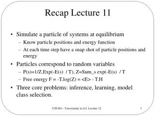
Recap Lecture 11 • Simulate a particle of systems at equilibrium • Know particle positions and energy function • At each time step have a snap shot of particle positions and energy • Particles correspond to random variables • P(s)=1/Z.Exp(-E(s) / T), Z=Sum_s exp(-E(s) / T • Free energy F = -T.log(Z) = <E> - T.H • Three core problems: inference, learning, model class selection. CSI 661 - Uncertainty in A.I. Lecture 12
Base Problems To Solve • Calculating expectation of a function • Inference • Optimal Bayesian Classifier • Calculating maximum function value • Finding mode • Multiple modes • Figure 3.1 Neal CSI 661 - Uncertainty in A.I. Lecture 12
Stochastic Algorithmic Solutions • Numerical Methods: Exact solutions • Rejection sampling • Importance sampling • Methods to find the posterior mode • Markov Chain Monte Carlo Sampling CSI 661 - Uncertainty in A.I. Lecture 12
Markov Chains • Invariant/stationary distributions • Ergodic chains • Irreducible, aperiodic, one stationary distribution. • Computational perspective: • how quickly moves between states can be generated, • how quickly equilibrium is reached from any initial state, • the number of moves required to move from state x to a state y which is independent of x. CSI 661 - Uncertainty in A.I. Lecture 12
Markov Chains • A Markov chain consists of a series of random variables X(0), X(1), X(2), X(3), … X(t) • P(x(t+1) | x(t), x(t-1),x(t-2) … x(0)) = P(x(t+1) | x(t)). • X(0) is known as the initial distribution and the distribution for X(t+1) • We begin in a randomly drawn state from the initial distribution and move around the state space according to the state transition probabilities • Homogenous versus heterogeneous CSI 661 - Uncertainty in A.I. Lecture 12
Markov Chain Properties CSI 661 - Uncertainty in A.I. Lecture 12
Markov Chain Properties II • It will converge to the equilibrium distribution as t regardless of X(0) CSI 661 - Uncertainty in A.I. Lecture 12
Metropolis Algorithm CSI 661 - Uncertainty in A.I. Lecture 12
Hastings Generalization CSI 661 - Uncertainty in A.I. Lecture 12
BBN Learning Example CSI 661 - Uncertainty in A.I. Lecture 12
Statistical Physics - Background • Micro-state versus Macro-state • Micro-state unknown, partial knowledge • P(s) = 1/Z . Exp(-E(s) / T), Z = Sum_s exp(-E(s) / T • Known as the Gibbs, Boltzmann, canonical, equilibrium distribution • Equivalent to what? • Intensive versus Extensive quantities (grow linearly with system size) • Extensive quantities per unit/particle reach constant limits • Interested in systems at thermodynamic equilibrium • Macroscopic properties can be expressed as expectations CSI 661 - Uncertainty in A.I. Lecture 12
Ising Spin Glass Model Phase transitions CSI 661 - Uncertainty in A.I. Lecture 12
Free Energy of a SystemRelationship to A.I. • Free energy F = -T.log(Z) = <E> - T.H • Z is the partition function, T temperature • H the system entropy • F and H are extensive values • (cf. Slide 1) What are the analagous particles for: • Parameter estimation (learning) • Inference • Model class selection CSI 661 - Uncertainty in A.I. Lecture 12
Next Lecture • Read, Neal, Chapter 2 CSI 661 - Uncertainty in A.I. Lecture 12