The Basics
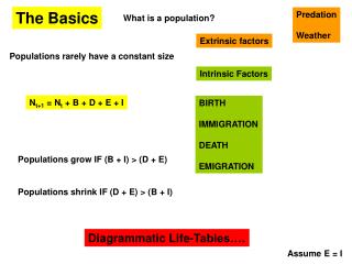
Predation Weather. Extrinsic factors. Intrinsic Factors. N t+1 = N t + B + D + E + I. BIRTH IMMIGRATION DEATH EMIGRATION. Populations grow IF (B + I) > (D + E). Populations shrink IF (D + E) > (B + I). The Basics. What is a population?. Populations rarely have a constant size.

The Basics
E N D
Presentation Transcript
Predation Weather Extrinsic factors Intrinsic Factors Nt+1 = Nt + B + D + E + I BIRTH IMMIGRATION DEATH EMIGRATION Populations grow IF (B + I) > (D + E) Populations shrink IF (D + E) > (B + I) The Basics What is a population? Populations rarely have a constant size Diagrammatic Life-Tables…. Assume E = I
Pods 18.25 Adults M F 2.5 2.5 7.3 11 Eggs 200.75 Adults Nt 0.079 f Instar I 15.86 Seeds Nt.f P=0 0.72 SURVIVAL g p BIRTH Instar II 11.42 Seedlings Nt.f.g 0.78 e Instar III 8.91 Adults Nt+1 Adults M F 2.3 2.3 0.76 0.69 Instar IV 6.77 Nt+1 = (Nt.p) + (Nt.f.g.e) t = 0 t = 0 t = 1 t = 1
Adults M F 5 5 10 Birth Birth Birth Eggs 50 0.84 a0 a1 a2 a3 an 1 mo Nestlings 42 t1 0.5 p23 p23 p12 p12 p01 p01 0.71 a0 a1 a2 a3 an 3 mo Fledglings 29.8 t2 0.1 Adults M F 8.2 8.2 a0 a1 a2 a3 an t3 Overlapping Generations: Discrete Breeding t1 t2 NB: Different age groups have different probabilities of surviving from one time interval to the next, and different age groups produce different numbers of offspring NB – ALL Adults or Females?
l refers to proportions wrt t0 – allows comparisons between cases: lx = ax / a0 Subscript x refers to age/stage class Conventional Life-Tables Best studied from Cohort – Define a refers to actual numbers counted – case specific
l refers to proportions wrt t0 – allows comparisons between cases: lx = ax / a0 Subscript x refers to age/stage class d refers to standardised mortality, calculated as lx – lx+1: data can be summed Conventional Life-Tables Best studied from Cohort – Define a refers to actual numbers counted – case specific
l refers to proportions wrt t0 – allows comparisons between cases: lx = ax / a0 Subscript x refers to age/stage class d refers to standardised mortality, calculated as lx – lx+1: data can be summed q age specific mortality, calculated as dx / lx: data cannot be summed Conventional Life-Tables Best studied from Cohort – Define a refers to actual numbers counted – case specific
l refers to proportions wrt t0 – allows comparisons between cases: lx = ax / a0 Subscript x refers to age/stage class d refers to standardised mortality, calculated as lx – lx+1: data can be summed q age specific mortality, calculated as dx / lx: data cannot be summed p age specific survivorship, calculated as 1 - qx (or ax+1 / ax): cannot be summed Conventional Life-Tables Best studied from Cohort – Define a refers to actual numbers counted – case specific
l refers to proportions wrt t0 – allows comparisons between cases: lx = ax / a0 Subscript x refers to age/stage class K d refers to standardised mortality, calculated as lx – lx+1: data can be summed q age specific mortality, calculated as dx / lx: data cannot be summed p age specific survivorship, calculated as 1 - qx (or ax+1 / ax): cannot be summed k killing power – reflects stage specific mortality and can be summed Conventional Life-Tables Best studied from Cohort – Define a refers to actual numbers counted – case specific
l refers to proportions wrt t0 – allows comparisons between cases: lx = ax / a0 Subscript x refers to age/stage class K d refers to standardised mortality, calculated as lx – lx+1: data can be summed q age specific mortality, calculated as dx / lx: data cannot be summed p age specific survivorship, calculated as 1 - qx (or ax+1 / ax): cannot be summed k killing power – reflects stage specific mortality and can be summed F Total number offspring per age/stage class Conventional Life-Tables Best studied from Cohort – Define a refers to actual numbers counted – case specific
l refers to proportions wrt t0 – allows comparisons between cases: lx = ax / a0 Subscript x refers to age/stage class K d refers to standardised mortality, calculated as lx – lx+1: data can be summed q age specific mortality, calculated as dx / lx: data cannot be summed p age specific survivorship, calculated as 1 - qx (or ax+1 / ax): cannot be summed k killing power – reflects stage specific mortality and can be summed F Total number offspring per age/stage class Conventional Life-Tables Best studied from Cohort – Define a refers to actual numbers counted – case specific m mean number offspring per individual a, Fx / ax
l refers to proportions wrt t0 – allows comparisons between cases: lx = ax / a0 REAL DATA Subscript x refers to age/stage class K d refers to standardised mortality, calculated as lx – lx+1: data can be summed q age specific mortality, calculated as dx / lx: data cannot be summed p age specific survivorship, calculated as 1 - qx (or ax+1 / ax): cannot be summed k killing power – reflects stage specific mortality and can be summed F Total number offspring per age/stage class lm number of offspring per original individual Conventional Life-Tables Best studied from Cohort – Define a refers to actual numbers counted – case specific m mean number offspring per individual a, Fx / ax
Σ lxmx = R0 = 0.51 N0 . R0 = 44000 . 0.51 = 22400 = NT Generation time Σ lxmx = R0 = ΣFx / a0 = Basic Reproductive rate R0 = mean number of offspring produced per original individual by the end of the cohort It indicates the mean number of offspring produced (on average) by an individual over the course of its life, AND, in the case of species with non-overlappinggenerations, it is also the multiplication factor that converts an original population size into a new population size – ONE GENERATION later R0 is a predictor that can be used to project populations into the future – in terms of generations
For populations with overlapping generations, we must tackle the problem in a roundabout manner Fundamental Reproductive Rate (R) = Nt+1 / Nt IF Nt = 10, Nt+1 = 20: R = 20 / 10 = 2 Populations will increase in size if R >1 Populations will decrease in size if R < 1 Populations will remain the same size if R = 1 R combines birth of new individuals with the survival of existing individuals R0 ONLY reflects the birth of new individuals (survival = 0) Population size at t+1 = Nt.R Population size at t+2 = Nt.R.R Population size at t+3 = Nt.R.R.R Nt = N0.Rt
Nt = N0.Rt Overlapping generations NT = N0.R0 Non-overlapping generations NT = N0.RT IF t = T, then R0 = RT lnR0 = T.lnR Can now link R0 and R: T = Σxlxmx / R0 T can be calculated from the cohort life tables X = age class lnR = r = lnR0 / T = intrinsic rate of natural increase
L average number of surviving individuals in consecutive stage/age classes: (ax + ax+1) / 2 n T cumulative L: ΣLx i e life expectancy: Tx / ax NB. Units of e must be the same as those of x Thus if x is measured in intervals of 3 months, then e must be multiplied by 3 to give life expectancy in terms of months Other statistics that you can calculate from basic life tables Life Expectancy – average length of time that an individual of age x can expect to live Can also calculate T and L using lx values T and L are confusing – call them Bob (L) and Margaret (T)
To convert FINITE rates at one scale to (adjusted) finite rates at another: [Adjusted FINITE] = [Observed FINITE] ts/to Where ts = Standardised time interval (e.g. 30 days, 1 day, 365 days, 12 months etc) to = Observed time interval e.g. convert annual survival (p) = 0.5, to monthly survival e.g. convert daily survival (p) = 0.99, to annual survival Adjusted = Observed ts/to Adjusted = Observed ts/to = 0.5 1/12 = 0.99 365/1 = 0.5 0.083 = 0.99 365 = 0.944 = 0.0255 A note on finite and instantaneous rates The values of p, q hitherto collected are FINITE rates: units of time those of x expressed in the life-tables (months, days, three-months etc) They have limited value in comparisons unless same units used
INSTANTANEOUS MORTALITY rates = Loge (FINITE SURVIVAL rates) ALWAYS negative Finite Mortality Rate = 1 – Finite Survival rate Finite Mortality Rate = 1.0 – e Instantaneous Mortality Rate MUST SPECIFY TIME UNITS
Dealing first with survivorship Copy Formula Down and Across Table quickly fills up with 0s Projecting Populations into the future: Basic Model Building KEY PIECES of INFORMATION: p and m Rearrange Life Table WHY?
Adding Fecundity 54256.42 Copy Down
R = (Nt+1) / Nt NB – R eventually stabilises Converting NUMBERS of each age class to PROPORTIONS (of the TOTAL) generates the age-structure of the population. NOTE, when R stabilises, so too does the age-structure, and this is known as the stable-age distribution of the population, and proportions represent TERMS (cx)
Calculating Birth Rate First n Divide by No Individuals producing them: Σax No Births = No a0 1 e.g. B = 35648277 / (1685933 + 80401 + 0) = 20.1821 Because the terms of the stable age distribution are fixed at constant R, we can partition r (lnR) into birth and death per individual Nt+1 = Nt.(Survival Rate) + Nt.(Survival Rate).(Birth Rate) Nt+1 = Nt.(Survival Rate).(1 + Birth Rate)
Calculating Survival Rate Survivors: Total number of individuals at time t, older than 0: n Σax Survival Rate: No Survivors at time t, divided by total population size at time t-1 1 e.g. Survival Rate (t4) = No survivors (t4) / total population size (t3) S = 348069 / 1452894 = 0.2396
At Stable-Age B = 20.1821 S = 0.2396 NOTE Annual Survival Rate for an individual in the population is in the range p0, p1, p2, but NOT the average Annual Birth Rate for an individual in the population is between m1 and m2, but NOT the average Nt+1 = Nt.(Survival Rate).(1 + Birth Rate) Nt+1 / Nt = R = er = (Survival Rate).(1 + Birth Rate) R = 0.2396 x (20.1821 + 1) = 5.07
This expression can ONLY be used to calculate vx* IF the time intervals used in the life-table are equal. vx = mx + vx* vx* = [(vx+1.lx+1) / (lx.R)] vx* = residual reproductive value To calculate vx* work backwards in the life-table, because vx* = 0 in the last year of life Copy upwards Reproductive Value (vx) – a measure of present and future contributions by the different age classes of a population to R vx is calculated as the number of offspring produced by an individual age x and older, divided by the number of individuals age x right now