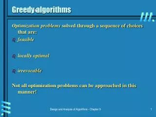
Greedy Algorithms
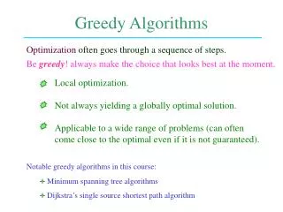
Local optimization. Not always yielding a globally optimal solution. Applicable to a wide range of problems (can often come close to the optimal even if it is not guaranteed). Notable greedy algorithms in this course:. Minimum spanning tree algorithms.

Greedy Algorithms
E N D
Presentation Transcript
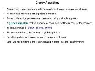
Local optimization. Not always yielding a globally optimal solution. Applicable to a wide range of problems (can often come close to the optimal even if it is not guaranteed). Notable greedy algorithms in this course: Minimum spanning tree algorithms Dijkstra’s single source shortest path algorithm Greedy Algorithms Optimization often goes through a sequence of steps. Be greedy!always make the choice that looks best at the moment.
incompatible events compatible (overlap) (no overlap) i k j s s f f j i i j Activity Selection Set S = {1, 2, …, n } of activities. time Problem: Find the largest set A of compatible events.
yes no S' = {iS | Sf } i 1 2 A ? 2 A ? S' yes no yes no S'' S'–{2} S'' S–{1,2} S'' = {iS | Sf } i 2 Overlapping Subproblems Recursively try all possible compatible subsets. 1 A ? S S–{1}
Greedy-Activity-Selector(s, f ) // (n)without the sorting n = length[s]; A = {1} j = 1 // last activity scheduled (current activity) fori = 2 ton do ifs f // next activity starts after current one finishes thenA = A + {i} j = i returnA i j // update the last scheduled activity A Greedy Solution // The input activities are in order by increasing finish time: ff … f // 1 2 n // Otherwise, sort them first.
incompatible – discard the event 2 1 Step 2 3 1 Step 3 4 compatible – schedule the event 1 4 Step 4 5 1 4 Step 5 6 A = {1, 4, 6} 1 4 6 schedule An Example 1 Step 1 0 1 2 3 4 5 6 7 8 9 10 11 12 13 14
k ... 1 ... Since ff , activities in A are compatible. Thus A is also optimal. 1 k Greedy Choice Claim1There exists an optimal schedule A S such that activity 1 is in A. Proof Suppose B S is an optimal schedule. There are two cases: (1) If 1 is in B then let A = B. (2) Otherwise, let k be the first activity in B Let A = B {k} + {1}:
B: ... A– {1}: ... 1 B + {1}: ... Optimal Substructure Claim 2 Let A be an optimal schedule, then A {1} is an optimal schedule for S' = { i in S | s f } i 1 Proof Suppose not true. Then there exists an optimal schedule B for S' with |B| > | A – {1} | = |A| – 1. Then the following solution to S has more activities than A. Contradiction.
In activity-selection Local optimal (greedy) choice → globally optimal solution Correctness of Greedy Algorithm Combine Claims 1 and 2 and induct on the number of choices: Theorem Algorithm Greedy-Activity-Selector produces solutions of maximum size for the activity-selection problem.
Both techniques rely on the presence of optimal substructure. The optimal solution contains the optimal solutions to subproblems. Dynamic programming solves subproblems first, then makes a decision. Greedy algorithm makes decision first, then solve subproblems.(Greedy-choice property gains efficiency.) Greedy Algorithm vs Dynamic Programming