Download
1 / 70
710 likes | 907 Vues
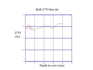
Bulk d 18 O thus far. d 18 O (‰). Depth in core (cms). Expected effect of temperature on the oxygen isotopic signal in calcite. Note the similarity to actual temperature (This means that the temperature effect on d 18 O usually dominates the salinity effect).

E N D
Bulk d18O thus far d18O (‰) Depth in core (cms)
Expected effect of temperature on the oxygen isotopic signal in calcite Note the similarity to actual temperature (This means that the temperature effect on d18O usually dominates the salinity effect)
Variables that must be considered • Solar irradience • albedo (snow and ice cover, including sea ice) • greenhouse gas content of atmosphere • surface temperature distribution • ocean heat transport (wind-driven and overturning) • winds
GISS atmospheric GCM results From J. Hansen, 2008
Descent of snowlines gives a sense of the temperature depression at higher elevations, at various latitudes
Most accessible example is Mauna Kea, Hawaii Glacial moraines can be Mapped about 800 meters Down from summit.
Modern distribution of sea surface temperature Surface of the ice age ocean reconstructed on the basis of changes in biogeography in sediment cores (CLIMAP project)
Biogeography of planktonic foraminifera in modern sediments. Examples shown here are “polar” (top panel) and “tropical” species. One can scale the relative abundance of these taxa to the temperature of the overlying waters. This is the basis for the so-called CLIMAP reconstruction of the ice age earth.
The assemblages in core top sediments are resolved into “factors” (principle components) and regressed onto observed sea surface temperature in the modern ocean
Descent of snowlines gives a sense of the temperature depression at higher elevations, at various latitudes
The climate sensitivity inferred from the last ice age depends critically on the temperature patterns assumed for the tropics CLIMAP results (from microfossil assemblages) New and improved CLIMAP Hostetler and Mix, Nature, 1999
Distribution of temperature observations from the Last Glacial Maximum East-west gradients reduced from Barrows et al. 2005
Fortunately, there are other means of deducing temperature in the ocean
Examples of Mg/Ca derived temperature From Lea, 2005
Gas chromatographic spectrum, showing the sensitivity of sedimentary alkenone unsaturation to temperature (T. Herbert, 1998)
“Unsaturation index” (ratio of di- and tri-unsaturated compounds to total)
Noble gases in aquifers give a measure of ground temperature variability
Water ages as it flows from recharge zone through the aquifer
Distribution of aquifers with glacial age water (and the inferences of temperature change from noble gas measurements)
Layer counting chronology can be extended to other archives by “wiggle matching” distinctive events
Example of changes in pollen assemblages in a famous European lake sediment core (Grande Pile)
The dynamics of continental vegetation might also create a feedback, through albedo effects. From “the Biome project” (animations are downloadable)
What about sea ice?(difficult to reconstruct directly, because not much sediment rains down from beneath sea ice)
Modern distribution of sea surface temperature Surface of the ice age ocean reconstructed on the basis of changes in biogeography in sediment cores (CLIMAP project)
Distribution of sea ice inferred from diatom taxa (Gersonde et al. 2004)
What about greenhouse gases?(measured directly from ice cores)
Antarctic + Greenland Temp. history methane N20 Ice core measurements of N2O over the last 80,000 years
What about strength of the sun?We don’t have any direct information, but we do know the distribution (seasonality) of solar radiation)
The direct effect of eccentricity is small. However, many climate records show considerable variability at frequencies matching the eccentricity cycle (413 ky and 96 kyr).
Precessional effects are complicated, because the two hemispheres are out of phase… However, the amplitude of the precessional cycle varies through time in a way that makes it a convenient “tuning fork”
Departure of incoming solar radiation as a function of latitude and orbital geometry (zero point is defined here as an arbitrary reference orbit)
GISS atmospheric GCM results From J. Hansen, 2008
Read it and weep, baby!!! d18O (‰) Depth in core (cms)
GISS atmospheric GCM results From J. Hansen, 2008
Once established, large ice sheets can create their own climate, to some extent.
A strategy that is now relatively common is to use coupled ocean atmosphere models of intermediate complexity to investigate the components of ice age cooling
Another example of a different model of intermediate complexity (from Weaver et al. 1998, Nature)
The global heat content of the ocean doesn’t change much in this model, even though the pattern of temperature change is disrupted. The implication from this model is that ocean circulation is not a real amplifier.
The various model results, though they deal with the surface of the ocean and atmosphere, raise the issue of what was happening in the deep ocean during the last ice age
Hydrography of the glacial ocean from Adkins et al., 2002, Science
Porewater profiles offer the opportunity to reconstruct LGM salinity from Adkins and Schrag, EPSL, 2003
How to separate the “ice volume effect” (i.e. sea level) from temperature in foram oxygen isotope records of the last ice age cycle Salinity (or d18O) measured in the sediment porewaters usually shows a remnant maximum some 30-50 meters below the sea floor. This maximum reflects the (now diffused) relict of when the oceans were last saltier--i.e. the last ice age. If diffusion rates of porewaters are known, and starting points are modelled, then one can reconstruct the salinity (or d18O composition) of the ocean during the last ice age. Schrag et al., Science, 1996