Download
1 / 10
110 likes | 391 Vues
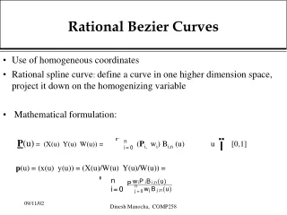
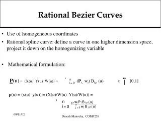
Rational Bezier Curves. Use of homogeneous coordinates Rational spline curve : define a curve in one higher dimension space, project it down on the homogenizing variable Mathematical formulation: P (u) = (X(u) Y(u) W(u)) = ( P i, w i ) B i,n (u) u [0,1]

E N D
Rational Bezier Curves • Use of homogeneous coordinates • Rational spline curve: define a curve in one higher dimension space, project it down on the homogenizing variable • Mathematical formulation: P(u) = (X(u) Y(u) W(u)) = (Pi, wi) Bi,n (u)u[0,1] p(u) = (x(u) y(u)) = (X(u)/W(u) Y(u)/W(u)) = Dinesh Manocha, COMP258
Rational Bezier Curves: Properties • Wi are the weights and they affect the shape of the curve • All the Wi cannot be simultaneously zero • If all the Wi are non-negative, the curve is still contained in the convex hull of the control polygon • It interpolates the end points • The tangents at P0 is givenby P1 - P0 and at Pn is givenby Pn - Pn-1 • The weights affect the shape in the interior. What happens when Wi • A rational curve has perspective invariance Dinesh Manocha, COMP258
Rational Bezier Curves and Conics • A rational Bezier curve can exactly represent a conic • The conics are second degree algebraic curve and their segments can be represented exactly using rational quadratic curves (i.e. 3 control points and 3 weights) • A parabola can be represented using a polynomial curve, but a circle, ellipse and hyperbola can only be represented using a rational curve Dinesh Manocha, COMP258
B-Spline Curves • Consists of more than one curve segment • Each segment is influenced by a few control points (e.g. local control) • Degree of a curve is indpt. of total number of control points • Use of basis function that have a local influence • Convex hull property: contained in the convex hull of control points • In general, it does not interpolate any control point(s) Dinesh Manocha, COMP258
Non-Uniform B-Spline Curves • A B-spline curve is defined as: • Each segment is influenced by a few control points (e.g. local control) where Pi are the control points, k controls the degree of the basis polynomials Dinesh Manocha, COMP258
Non-Uniform Basis Function • The basis function is defined as: where k controls the degree (k-1) of the resulting polynomial in u and also the continuity of the curve. • ti are the knot values, and a set knot values define a knot vector Dinesh Manocha, COMP258
Non-Uniform Basis Function • The parameters determining the number of control points, knots and the degree of the polynomial are related by where T is the number of knots. For a B-spline curve that interpolates P0 and Pn, the knot T is given as where the end knots and repeat with multiplicity k. • If the entire curve is parametrized over the unit interval, then, for most cases =0 and = 1. If we assign non-decreasing values to the knots, then =0 and = n –k + 2. where k controls the degree (k-1) of the resulting polynomial in u and also the continuity of the curve. ti are the knot values, and a set knot values define a knot vector Dinesh Manocha, COMP258
Non-Uniform Basis Function • Multiple or repeated knot-vector values, or multiply coincident control point, induce discontinuities. For a cubic curve, a double knot defines a join point with curvature discontinuity. A triple knot produces a corner point in a curve. • If the knots are placed at equal intervals of the parameter, it describes a UNIFORM non-rational B-spline; otherwise it is non-uniform. • Usually the knots are integer values. In such cases, the range of the parameter variable is: Dinesh Manocha, COMP258
Locality • Each segment of a B-spline curve is influenced by k control points • Each control point only influences only k curve segments • The interior basis functions (not the ones influenced by endpoints) are independent of n (the number of control points) • All the basis functions add upto 1: convex hull property Dinesh Manocha, COMP258
Uniform B-Spline Basis Functions • The knot vector is uniformly spaced • The B-spline curve is an approximating curve and not interpolating curve • The B-spline curve is a uniform or periodic curve, as the basis function repeats itself over successive intervals of the parametric variable • Use of Non-uniformity: insert knots at selected locations, to reduce the continuity at a segment joint Dinesh Manocha, COMP258