The Solar Wind and Heliosphere
820 likes | 1.29k Vues
The Solar Wind and Heliosphere. Bob Forsyth - 3 rd December 2012. TOPICS The Sun – interior and atmosphere Origin of the solar wind Formation of the heliosphere Outer boundaries of the heliosphere Heliospheric spacecraft The heliospheric magnetic field Fast and slow solar wind flows

The Solar Wind and Heliosphere
E N D
Presentation Transcript
The Solar Wind and Heliosphere Bob Forsyth - 3rd December 2012 TOPICS The Sun – interior and atmosphere Origin of the solar wind Formation of the heliosphere Outer boundaries of the heliosphere Heliospheric spacecraft The heliospheric magnetic field Fast and slow solar wind flows Evolution with the solar cycle Corotating Interaction Regions Coronal Mass Ejections
Overview of solar interior and atmosphere Priest (1995)
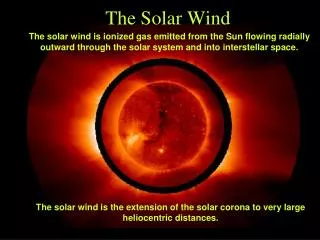
The solar wind • The solar wind, consisting of ionised coronal plasma, flows supersonically and radially outward from the Sun due to the large pressure difference between the hot solar corona and the interstellar medium. Property at 1 AU Speed (v) ~400 km/s Number density (n) ~10 cm–3 Flux (nv) ~3108 cm–2 s–1 Magnetic field (Br) ~3 nT Proton temperature (Tp) ~4104 K Electron temperature(Te) ~1.3105 K (>Tp) Composition (He/H) ~1 – 30% + trace heavier elements
Parker model of the solar wind • Parker(1958) was the first to propose a model of the solar wind assuming a steady flow of plasma independent of time, as opposed to a static corona. • He began from the mass and momentum conservation equations, taking time derivatives as zero since considering a steady flow… • Assuming isothermal and B=0 he found a solution of the form…
Parker solar wind solutions for a range of temperatures Parker (1958)
Early solar wind observations from Mariner 2 in 1962 Hundhausen (1995)
Weber and Davis (1967) derived a model which included the magnetic field – this leads to additional critical points in the equations
The Heliosphere • The heliosphere is the volume of space, enclosed within the interstellar medium, formed by, and which contains, the outflowing solar wind and the Sun's magnetic field. • The size of the heliosphere, known to be more than 100 AU, is determined by a balance between the dynamic pressure of the solar wind and the pressure of the interstellar medium.
Outer boundaries of the heliosphere • The boundary between the solar wind plasma and interstellar plasma is known as the ‘heliopause’. • Because the solar wind flow is supersonic it cannot ‘sense’ that it is approaching the heliopause. Thus a standing shock wave, the ‘termination shock’, must form at some distance inside the heliopause so that the flow is slowed to subsonic speeds. • The solar wind plasma can then be deflected in the region between the termination shock and the heliopause to flow down the ‘heliotail’. • Due to the motion of the heliosphere through the interstellar medium, the interstellar plasma is deflected to flow round the outside of the heliopause. • Depending on the speed of this motion, a bow shock may form in the interstellar medium upstream of the heliopause.
Heliospheric Spacecraft • The first observations of the solar wind were made in the vicinity of the Earth in the early 1960s. • Pioneer 10 and 11, launched in 1972 and 1973 were the first spacecraft to explore beyond 1 AU. Contact with these spacecraft have now been lost although Pioneer 10 was tracked to nearly 80 AU. • Voyager 1 and 2 were launched in 1977. Both have scientific instruments still operating. Voyager 1 crossed the termination shock in 2004 at 94.5 AU, has now reached 123 AU and continues out towards the heliopause. Voyager 2, following behind, crossed the termination shock at 84 AU in 2007. • Helios 1 and 2, launched in 1974 and 1976, explored the inner heliosphere in the ecliptic plane between 0.3 and 1 AU from the Sun. • Ulysses, launched in 1990 into a ~6 year period orbit of the Sun inclined at 80.2° to the solar equator, with perihelion at 1.3 AU and aphelion at 5.4 AU. It was thus the first spacecraft to explore the 3D structure of the heliosphere over a large latitude range. Operations ceased in 2009 after nearly 3 orbits. • STEREO, launched in 2006, consists of two spacecraft at 1 AU separating in solar longitude ahead of and behind the Earth. They carry instrumentation aimed at obtaining stereoscopic views of the Sun and to make multi-point in-situ measurements of the solar wind.
The heliospheric magnetic field • The heliospheric magnetic field is a result of the Sun’s magnetic field being carried outward, frozen in to the solar wind. • Within the corona, the magnetic field forces dominate the plasma forces. • As the field strength decreases with distance, beyond the Alfvén radius at a few solar radii, the plasma flow becomes dominant, and the field lines are constrained to move with the solar wind. Model of Pneumann and Kopp (1971)
For modelling purposes, a ‘source surface’ is assumed, typically ~2.5 solar radii, at which the magnetic field lines are constrained to be radial. (http://wso.stanford.edu/)
Examples of potential field models of the corona… Bravo et al (1998)
The heliospheric current sheet forms where outward field lines from one hemisphere meet inward field lines from the other hemisphere.
Near solar minimum when the Sun’s dipole field is dominant, the current sheet can be viewed as a plane tilted at the same angle as the dipole, embedded in the band of slow solar wind. • Therefore interplanetary spacecraft observe current sheet crossings up to a latitude equal to the dipole tilt angle. Smith (1997)
Ulysses passages above the maximum latitude of the current sheet…
The current sheet mapped out into the heliosphere… Jokipii and Thomas (1981)
The Parker Spiral Field • The solar magnetic field is frozen in to the radial outflowing solar wind. Thus, due to the Sun’s rotation, the magnetic field lines adopt an Archimedean spiral configuration. • The angle to the radial direction of the magnetic field depends on distance, latitude and the local solar wind velocity. Parker (1963)
Geometry of the Parker Field • The radial component of the magnetic field can be shown from flux conservation to depend only on distance: • Br(r,q,f) = Br(r0,q,f0)(r0/r)2 • By considering the relative motion of a solar wind plasma parcel and its source point, the equation for the spiral field lines is obtained: • r – r0 = –(f – f0) Vr / sinq • From this it can be shown that the azimuthal component goes as 1/r: • Bf(r,q,f) = –Br(r0,q,f0) sinq r02 / Vrr • Also Bq(r,q,f) = 0
Measurements near the ecliptic plane are found to fit this picture to a good approximation. Forsyth et al (1996)
Moving away from the equator, field lines gradually become less tightly wound with latitude until a field line originating exactly from the pole remains purely radial. • Ulysses showed that this was followed to a good first approximation also at high latitudes.
In an attempt to explain Ulysses energetic particle fluxes at high latitudes a more complex field model was proposed by Fisk and co-workers. Fisk (1996) Fisk and Jokipii (1999)
Others argue that the particles reach high latitudes as a result of field line mixing due to the random motion of footpoints in the corona… Jokipii and Kota (1989) Giacalone (1999)
Dependence of Field Strength on Latitude • Assuming that the magnetic field is radial at the ‘source surface’, the radial component of the magnetic field can be used to infer the field strength near the Sun since r2Br is a constant. • Ulysses observations showed that r2Br had no dependence on latitude. • This implies that the latitudinal magnetic pressure gradient associated with strong photospheric polar fields must have relaxed by the outer corona. Smith and Balogh (1995)
r2Br from Ulysses first fast latitude scan at solar minimum Forsyth et al (1996)
Comparing r2Br from Ulysses one solar minimum apart… Reduction of ~34%
South North Smoothed average 2006 1976 1988 2000 1982 1994 Photospheric field also reduced… Wilcox Solar Obsevatory (http://wso.stanford.edu)
At the recent solar minimum the heliospheric magnetic field at 1 AU was at the lowest since spacecraft records began… Owens et al (2008)
…and the solar wind was at its weakest in the space age McComas et al (2008)
Fast and Slow Solar Wind • Since the first spacecraft observations it was known that the solar wind was divided into streams of slow (~400 km/s) and fast (>500 km/s) wind. Hundhausen (1995)
Ulysses found continuous fast solar wind (~750 km/s) at high latitudes at solar minimum in agreement with the idea that fast solar wind originated in coronal holes. This fast wind was associated with large stable polar coronal holes. • Slow solar wind is associated with the streamers seen in coronagraph images, but its exact source is unclear. McComas et al (1998)
Close to solar minimum the flow pattern close to the Sun can be approximated as a band of slow wind at low latitudes, centred on the Sun’s dipole equator, with fast wind at all higher latitudes. • This pattern of fast and slow solar wind is occasionally disturbed by transient flows associated with coronal mass ejections. Pizzo (1991)
Characteristics of slow and fast solar wind Property at 1 AU Slow wind Fast wind Speed (v) ~400 km/s ~750 km/s Number density (n) ~10 cm–3 ~3 cm–3 Flux (nv) ~3108 cm–2 s–1 ~2108 cm–2 s–1 Magnetic field (Br) ~3 nT ~3 nT Proton temperature (Tp) ~4104 K ~2105 K Electron temperature(Te) ~1.3105 K (>Tp) ~1105 K (<Tp) Composition (He/H) ~1 – 30% ~5%
Solar cycle evolution • The tilt of the underlying solar dipole field and hence of the heliospheric current sheet and the band of slow wind is a function of the solar cycle, with least tilt near solar minimum. • Alternatively, the evolution of the coronal field can be viewed as the strength of the dipole component decreasing as solar activity increases so that the higher order components of the solar field have a greater effect. Suess et al (1998)
This evolution culminates in the reversal of the Sun’s magnetic field during the solar maximum period.
At solar maximum the large polar coronal holes disappear and are replaced by smaller, generally short lived coronal holes at all latitudes. Ulysses observed fast and slow wind at all latitudes in the southern hemisphere. McComas et al, (2008)
Corotating Interaction Regions • Interaction regions form wherever fast solar wind ‘catches up’ with slower wind ahead of it. • A compression region forms where the magnetic field lines and plasma ‘pile up’. The resulting pressure waves can steepen into shocks. • When a fast solar wind stream originates from a stable coronal hole persisting over many solar rotations, the resulting interaction region pattern corotates with the Sun. • Ulysses provided new results on the three dimensional geometry of Corotating Interaction regions. Pizzo (1985)
Interaction Regions in 1D • Because of the Sun’s rotation faster plasma emitted along a particular radial line, catches up with slower plasma emitted in the same direction at an earlier time. • The plasma streams cannot interpenetrate because of the frozen in magnetic field. • A compression region builds up leading the fast stream, while a rarefaction develops behind. • Due to pressure gradients the compression region expands at the fast mode speed. A forward wave develops on the leading edge and a reverse wave on the trailing edge. Gosling (1998)