Understanding Scientific Visualization: A Guide for Biological and Physical Scientists
630 likes | 779 Vues
This seminar, led by Robert Moorhead from Mississippi State University, aims to introduce the fundamentals of Scientific Visualization (SV) to biological and physical scientists with minimal computing experience. Participants will learn how SV methods transform numerical data into geometric representations, enhancing understanding of complex biological and physical processes. The session will cover the potential applications and limitations of SV in biomedical computing while emphasizing the importance of visual data analysis in scientific inquiry and discovery.

Understanding Scientific Visualization: A Guide for Biological and Physical Scientists
E N D
Presentation Transcript
Scientific Visualization for Biological and Physical Scientists Robert Moorhead Director Visualization, Analysis, and Imaging Lab Engineering Research Center Mississippi State University
My Charge • A seminar on “Sci Viz for Dummies”. • Explain what SV methods are and represent in regard to physical and biological processes, and how they are handled on computers. • The level should be very deliberately low, hoping to inform biological (especially) and physical scientists with little computing experience of the potential and limitations of SV methods in biomedical computing, and how they can thus be used.
What is Scientific Visualization? • the mapping of data and/or information to images to gain or present understanding and insight • the visual analysis of scientific data. It transforms the numeric representation into a geometric (image) representation, enabling a scientist, engineer, or mathematician to observe his simulated or measured data • Scientific Visualization encompasses and unifies the fields of computer graphics, image processing, computer vision, computer-aided design, signal processing, and human-computer interaction • Scientific Visualization is a set of software tools coupled with a powerful 3D graphical computing environment that allows any geometric object or concept to be visualized by anyone. The software provides an easy to use interface for the user. The hardware must be able to manipulate complex, geometrically-described, 3D environments in motion, color, and with any level of “realism” called for to better communicate the essence of the computation (in foreword of An Introductory Guide to Scientific Visualization. R. A. Earnshaw & N. Wiseman, Springer-Verlag, 1992) • SciVi, SciViz, SciVis, SV, ...
Why Scientific Visualization? • “The purpose of computing is insight, not numbers” Richard Hamming (1962) • “Maintain a Healthy Skepticism: Never believe the results of your calculations. Always look for errors, limitations, unnatural constraints, inaccurate inputs, and places where algorithms break down. Nothing works until it is tested, and it probably does not really work even then. This skepticism should help avoid embarrassing situations, such as occur when a neat physical explanation is painstakingly developed for a computational blunder.” E. S. Oran & J. P. Boris (1987) • “In decreasing order of importance, scientific visualization: - shows you where you are screwing up - allows discoveries - is useful for show-and-tell” J. J. O’Brien (1993)
Why Scientific Visualization? • to assist existing scientific processes by providing new insight through visual representation • The visual sensory path is the widest information pipeline to the brain • A picture is worth a thousand words (or about 6000 numbers) • To see your mistake: • not checking the return code when reading data • zero length or truncated record is read • set of values reused or used incorrectly • The human mind is particularly effective at abstraction, approximation and simplification. Visualization, historically, is an internal mental process. E.g., I see what you are talking about, see what I mean? • One of the reasons for scientific (data, computational) visualization is the complexity or quantity of the data (or both) make it impossible to comprehend or manipulate more than a small portion of the model or data space internally at a given instant. • With scientific visualization, data can be • graphically elaborated (rendered), or • explored (segmented, sliced, recolored, rotated, flown around, etc.)
Visualization Goals • Comparing: images, positions, data sets, subsets of data. • Distinguishing: importance, objects, activities, range of value. • Indicating directions: orientations, order, direction of flow. • Locating: position relative to axis, object, map. • Relating: concepts, e.g. value and direction, position and shape, temperature and velocity, object type and value. • Representing values: numeric value of data. • Revealing objects: exposing, highlighting, bringing to the front, making visible, enhancing visibility.
Types of Scientific Visualization • I See • interactive • exploratory • softcopy display • minimal contextual information • We See • interactive • exploratory • softcopy display • more context/explanation needed • They See • presentation usually • not interactive • not exploratory • hardcopy display • lots of context/explanation needed
Scientific Visualization: Why?Insight • ribbon diagram of the 4mdh protein from the Protein Data Bank SDSC: P. Bourne, M. Gribskov, J. Moreland, G. Johnson, H. Weissig
Scientific Visualization: Why?Insight • Computed Tomography and microtomed traversal data from the Visible Human Project • SDSC: J. Genetti, G. Johnson
Scientific Visualization Process Summarize Data Source Filter Playback Data Data Images Render Mapping Mapping Geometric Primitives
Types of Source Data • Measured (sensed, observed, experimental) • Simulated (computed)
Measured or Computed? • Is that really measured data? ….
Dimensions • domain (independent variables) • 2D, 3D, 4D, etc. • if the data points are not connected: scattered • if the domain is gridded: • rectilinear (uniform [regular] or non-uniform [irregular]) • cubes: with data points at vertices, on faces, or in the center • curvilinear • distorted cubes, but 6-connectivity at nodes, analogy is a distorted sponge • unstructured • 2D - triangles • 3D – tetrahedra, prisms, pyramids, or hexahedra • range (dependent variables) • scalar (pressure, density, temperature, voltage, height, salinity) • vector (velocity, current, gradient, etc.) • tensor (stress, strain, etc.)
How to turn data into an image • Ultimately you turn on a discrete point on the computer screen or you put a finite quantity of colored material on some material or …wet chemistry. • You have to make a lot of choices in how you want that done. • The process can be divided in mathematical steps, scientific steps, and engineering steps. • I’m not going to go any deeper now; let’s look at some methods …
Classes of Visualization Techniques • Glyph techniques – use symbols to represent values or states within a field of information. • Surface Methods – extracts polygonal versions of calculated components. • Direct Volume Rendering – generates a rendered image of the volume where volume elements are projected directly onto the image plane.
Surface Methods • Cutting Planes • Isosurfaces • Direct Volume Rendering
Techniques for Scalar Entities Three-Dimensional Domain • F(x1,x2,x3) • These techniques are often called volume visualization • Two major approaches will be described: • one produces isosurfaces (surface rendering) • the other is direct volume rendering (DVR), which attempts to display the “whole” volume in one image (volume rendering)
Techniques for 3D Scalar Entities (cont.) • Isosurfaces: • The three steps to isosurface construction are: • detect surface(s) • fit geometric primitives to the detected surface(s) • render surface • two methods for fitting geometric primitives: • contour connection methods • voxel intersection methods • dividing cubes • marching cubes • Marching Cubes works by classifying the eight nodes of a voxel as being greater-than or less-than a threshold. These eight bits are used as an index into an edge intersection table. Linear interpolation is used to determine edge-intersection location and triangles are fitted to the edges. The triangles and the surface normals at vertices are added to a linked list for rendering.
Marching Cubes Linear on Edges:
Techniques for 3D Scalar Entities (cont.) • We want to map data from a 3D world onto a 2D plane • Volume visualization is the process of displaying values defined in 3-space, i.e., f(x,y,z). • Volume rendering in general has large computational and memory requirements. • Animation is crucial to the volume visualization process; seldom are the other visual cues sufficient to successfully comprehend the 3D structure of the volume. • Three Approaches • surface-fitting (SF) • direct volume rendering (DVR) • a combination -- cast rays through a thresholded data volume
Techniques for 3D Scalar Entities (cont.) DVR or Ray Casting:
Techniques for 3D Scalar Entities (cont.) • The objective of direct volume rendering is to display a scalar field of gridded data in a single image, as opposed to those techniques which display only a subset of the field, e.g., cutting planes and isosurfaces. • Color and opacity are assigned to each possible voxel value via classification tables (usually accessed with transfer functions). • Images are formed by blending together voxels projecting to the same pixel on the image plane. • Voxels may be projected in either object order or image order. • Sampling along a viewing ray often requires resampling, i.e., finding a value between voxel nodes. Nearest-neighbor, tri-linear interpolation, or tri-cubic interpolation are used, based on a speed/quality trade-off. • Gradients are used to approximate surface normals and are usually found using central difference.
Techniques for 3D Scalar Entities (cont.) • The amount of structure in the dataset usually determines which volume visualization algorithm will create the most informative images. Volume Characteristics Voxels and Cells • Volumes of data can be treated as either an array of volume elements (voxels) or an array of cells. • voxel - the area around a data point
Techniques for 3D Scalar Entities (cont.) • cell - views volume as a collection of hexahedra whose corners are the data points • Almost every volume visualization algorithm requires resampling which requires interpolation (or reconstruction). Common steps in volume visualization algorithms • data acquisition • slice processing • dataset reconstruction • dataset classification • mapping into primitives
Techniques for 3D Scalar Entities (cont.) Data Classification •most difficult task • choose threshold if SF algorithm • choose color and opacity for range of data values if DVR • other factors • user’s knowledge of the material (data) being visualized • if the f(x) are density values and you know bone has a density of 0.8 and you want to see bone, you set the opacity of f(x)=0.8 to 1.0 • the location of the classified elements in the volume • often want outer layers more transparent, thus element position is factored into the formula • the material occupancy of the element • When the data values are changing slowly, only a narrow range of values is acceptable as the isovalue surface. When the data values are changing rapidly, a wide range of values is acceptable as the isovalue surface.
Techniques for 3D Scalar Entities (cont.) Traversals • image-order - for each pixel see what objects (elements) project onto the pixel (remember, a pixel covers an area on the screen). • object-order - for each object (element) see where it intersects the image plane • can progress front-to-back (saves some computation potentially), or • back-to-front (can see scene evolve)
Techniques for 3D Scalar Entities (cont.) Viewing and Shading • many DVR algorithms allow only orthographic viewing since perspective viewing has ray divergence problems • SF algorithms can use either: • advantage of perspective: realistic view • advantage of parallel: no warping • both DVR and SF use gradient shading • once the gradient (or surface normal) is known, most shading algorithms can be used (flat, Gouraud, Phong, etc.) • all types of lighting are used (see chapter 16 of Foley et al ’95 or OpenGL Programming Guide for more details on shading): • ambient - depends on material property; intrinsic intensity (uniform) • diffuse - dependent on direction and distance • specular - highlights when view angle and reflection angle align
Techniques for 3D Scalar Entities (cont.) • gradient shading is usually more accurate than using the normals of the surface primitives • shading is an important factor in creating understandable volume images, however, sometimes you can shade too much
Techniques for 3D Scalar Entities (cont.) Photorealism • Photorealism is a hotly debated issue in DVR. The issue is should objects look like they are made from “real” material? The problem is that plausible objects may be misleading, but non-plausible may be hard to interpret. No consensus exists.
Techniques for 3D Scalar Entities (cont.) Direct Volume Visualization Algorithms • ray casting • image-order traversal • find color and opacity for each pixel by accumulating opacities and shaded colors along the ray • differs from ray-tracing in that there are no reflections (or refractions usually) • continue to cast the ray until the ray contents sum to unity or until the ray exits the volume • rather CPU intensive
Techniques for 3D Scalar Entities (cont.) • affine transform methods • feed-forward algorithm • warp slices or volumes into the image plane using affine transformations • warp the data until the data samples become pixel-aligned • then scan each data column of pixels and determine the pixel’s color • want to make all the magnification passes before the minification passes • splatting • front-to-back (or back-to-front) object-order traversal of the volume contents • like throwing a snowball at a glass plate • contribution is high in center; falls off near edges of footprint
Techniques for 3D Scalar Entities (cont.) • frequency domain volume rendering (or Fourier volume rendering) • uses the Fourier Projection-Slice Theorem • can obtain an image for any view direction and orientation by extracting a 2D plane of data from a 3D Fourier-transformed volume of data and just inverse transforming the slice of data. • limitation: the projections lack depth information (like an x-ray), but people have developed some methods to produce some lighting and depth cueing. • limitation: requires significant interpolation & reconstruction processing • easier to generate progressive refinements than with spatial techniques • spatial filtering is trivial to implement