Practical Methodology for Hyperparameter Optimization in Autoencoders
480 likes | 581 Vues
Learn about performance metrics, hyperparameter selection, debugging strategies, and practical examples for multi-digit number recognition in neural networks. Understand factors driving success in machine learning and how to choose the right architecture family. Discover ways to build end-to-end systems and adapt based on data-driven insights.

Practical Methodology for Hyperparameter Optimization in Autoencoders
E N D
Presentation Transcript
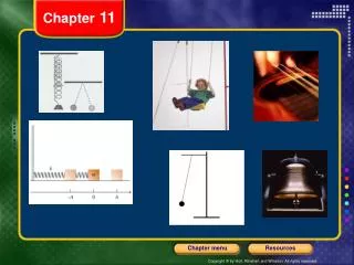
Goodfellow: Chapter 11Practical Methodology Dr. Charles Tappert The information here, although greatly condensed, comes almost entirely from the chapter content.
Chapter 11 Sections • Introduction • 1. Performance Metrics • 2. Default Baseline Models • 3. Determining Whether to Gather More Data • 4. Selecting Hyperparameters • 4.1 Manual Hyperparameter Tuning • 4.2 Automatic Hyperparameter Optimization Algorithms • 4.3 Search • 4.4 Random Search • 4.5 Model-Based Hyperparameter Optimization • 5. Debugging Strategies • 6. Example: Multi-Digit Number Recognition
Introduction • An autoencoder is a neural network trained to copy its input to its output • Network has encoder and decoder functions • Autoencoders should not copy perfectly • But restricted by design to copy only approximately • By doing so, it learns useful properties of the data • Modern autoencoders use stochastic mappings • Autoencoders were traditionally used for • Dimensionality reduction as well as feature learning
WhatdrivessuccessinML? Arcane knowledge of dozens of obscure algorithms? Knowing how to apply 3-4 standard techniques? Mountains of data? (2) (2) (2) h1 h2 h3 (1) (1) (1) (1) h1 h2 h3 h4 v1 v2 v3 (Goodfellow2016)
Example: Street View Address Number Transcription (Goodfellowetal,2014) (Goodfellow2016)
ThreeStepProcess Useneedstodefinemetric-basedgoals • Buildanend-to-endsystem • Data-drivenrefinement • (Goodfellow2016)
IdentifyNeeds Highaccuracyorlowaccuracy? • Surgeryrobot:highaccuracy • Celebritylook-a-likeapp:lowaccuracy • (Goodfellow2016)
ChooseMetrics Accuracy? (%ofexamplescorrect) • Coverage? (%ofexamplesprocessed) • Precision? (%ofdetectionsthatareright) • Recall? (%ofobjectsdetected) Amountoferror?(Forregressionproblems) • • (Goodfellow2016)
End-to-endSystem GetupandrunningASAP • Buildthesimplestviablesystemfirst • Whatbaselinetostartwiththough? • Copystate-of-the-artfromrelatedpublication • (Goodfellow2016)
DeeporNot? Lotsofnoise,littlestructure->notdeep • Littlenoise,complexstructure->deep • Goodshallowbaseline: • Usewhatyouknow • Logistic regression, SVM, boosted tree are all good • (Goodfellow2016)
ChoosingArchitectureFamily Nostructure->fullyconnected • Spatialstructure->convolutional • Sequentialstructure->recurrent • (Goodfellow2016)
FullyConnectedBaseline 2-3hiddenlayerfeed-forwardneuralnetwork • AKA“multilayerperceptron” • V Rectifiedlinearunits • W Batchnormalization • Adam • Maybedropout • (Goodfellow2016)
ConvolutionalNetworkBaseline Downloadapretrainednetwork • Orcopy-pasteanarchitecturefromarelatedtask • Or: • Deepresidualnetwork • Batchnormalization • Adam • (Goodfellow2016)
RecurrentNetworkBaseline output × LSTM • outputgate self-loop SGD • + × state forgetgate Gradientclipping • × inputgate Highforgetgatebias • input (Goodfellow2016)
Data-drivenAdaptation Choosewhattodobasedondata • Don’tbelievehype • Measuretrainandtesterror • “Overfitting”versus“underfitting” • (Goodfellow2016)
HighTrainError Inspectdatafordefects • Inspectsoftwareforbugs • Don’t roll your own unless you know what you’re doing • Tunelearningrate(andotheroptimizationsettings) • Makemodelbigger • (Goodfellow2016)
CheckingDataforDefects Canahumanprocessit? • 26624 (Goodfellow2016)
IncreasingDepth EffectofDepth 96.5 96.0 95.5 95.0 94.5 94.0 93.5 93.0 92.5 Testaccuracy(%) 92.0 3 4 5 6 7 8 Number of hidden layers 9 10 11 (Goodfellow2016)
HighTestError Adddatasetaugmentation • Adddropout • Collectmoredata • (Goodfellow2016)
IncreasingTrainingSetSize 20 Bayes error Train (quadratic) Test (quadratic) Test (optimal capacity) Train (optimal capacity) 6 degree) 5 15 (polynomial 4 10 3 (MSE) Error Optimalcapacity 2 5 1 0 0 100 101 102 103 #trainexamples 104 105 100 101 102 103 #trainexamples 104 105 (Goodfellow2016)
TuningtheLearningRate 8 7 6 5 4 3 2 1 Trainingerror 0 10-2 10-1 Learningrate(logarithmicscale) 100 Figure11.1 (Goodfellow2016)
Reasoning about Hyperparameters Hyperparameter Increases capacity when. . . Reason Caveats Number of hid- den units increased Increasing the number of hidden units increases the representational capacity of the model. Increasing the number of hidden units increases both the time and memory cost of essentially every op- eration on the model. Table11.1 (Goodfellow2016)
HyperparameterSearch Grid Random Figure11.2 (Goodfellow2016)
1. Undercomplete Autoencoders • There are several ways to design autoencoders to copy only approximately • The system learns useful properties of the data • One way makes dimension h < dimension x • Undercomplete: h has smaller dimension than x • Overcomplete: h has greater dimension than x • Principle Component Analysis (PCA) • An undercomplete autoencoder, linear decoder and MSE loss function, learns same subspace as PCA • Nonlinear encoder/decoder functions yield more powerful nonlinear generalizations of PCA
AvoidingTrivialIdentity Undercompleteautoencoders • hhaslowerdimensionthanx • forghaslowcapacity(e.g.,linearg) • Mustdiscardsomeinformationinh • Overcompleteautoencoders • hhashigherdimensionthanx • Mustberegularized • (Goodfellow2016)
2. Regularized Autoencoders • Allow overcomplete case but regularize • Use a loss model that encourages properties other than copying the input to the output • Sparsity of representation • Smallness of the derivative of the representation • Robustness to noise or missing inputs
3. Representational Power, Layer Size, and Depth • Autoencoders are often trained with only a single layer encoder and a single layer decoder • Using deep encoders and decoders offers the advantages of usual feedforward networks
4. Stochastic Encoders and Decoders • Modern autoencoders use stochastic mappings • We can generalize the notion of the encoding and decoding functions to encoding and decoding distributions
StochasticAutoencoders h pencoder(h | x) pdecoder(x | h) x r Figure14.2 (Goodfellow2016)
5. Denoising Autoencoders • A denoising autoencoder (DAE) is one that receives a corrupted data point as input and is trained to predict the original, uncorrupted data point as its output • Learn the reconstructed distribution • Choose a training sample from the training data • Obtain corrupted version from corruption process • Use training sample pair to estimate reconstruction
DenoisingAutoencoder h g f x˜ L C:corruptionprocess (introducenoise) C(x˜| x) L=-logpdecoder(x|h=f(x˜)) x Figure14.3 (Goodfellow2016)
Denoising Autoencoders Learn a Manifold Gray circle of equiprobable corruptions x˜ g o f x˜ C(x˜| x) Corrupted point falls back to nearest point on the manifold Figure14.4 (Goodfellow2016)
Vector Field Learned by a Denoising Autoencoder (Goodfellow2016)
6. Learning Manifolds with Autoencoders • Like other machine learning algorithms, autoencoders exploit the idea that data concentrates around a low-dimensional manifold • Autoencoders take the idea further and aim to learn the structure of the manifold
Tangent Hyperplane of a Manifold Amount of vertical translation defines a coordinate along a 1D manifold tracing out a curved path through image space Figure14.6 (Goodfellow2016)
Learning a Collection of 0-D Manifolds by Resisting Perturbation 1.0 Identity Optimalreconstruction 0.8 0.6 0.4 0.2 r(x) 0.0 x1 x0 x2 x Reconstruction invariant to small perturbations near data points Figure 14.7 (Goodfellow2016)
Non-Parametric Manifold Learning with Nearest-Neighbor Graphs Figure14.8 (Goodfellow2016)
Tiling a Manifold with Local Coordinate Systems Each local patch is like a flat Gaussian “pancake” Figure14.9 (Goodfellow2016)
7. Contractive Autoencoders • The contractive autoencoder (CAE) uses a regularizer to make the derivatives of f(x) as small as possible • The name contractive arises from the way the CAE warps space • The input neighborhood is contracted to a smaller output neighborhood • The CAE is contractive only locally
ContractiveAutoencoders @f(x)2 ⌦(h) = A . (14.18) F @x Input point Tangentvectors Local PCA(nosharingacrossregions) Contractiveautoencoder Figure14.10 Dog from CIFAR-10 dataset (Goodfellow2016)
8. Predictive Sparse Decomposition • Predictive Sparse Decomposition (PSD) is a model that is a hybrid of sparse coding and parametric autoencoders • The model consists of an encoder and decoder that are both parametric • Predictive sparse coding is an example of learned approximate inference (section 19.5)
9. Applications of Autoencoders • Autoencoder applications • Feature learning • Good features can be obtained in the hidden layer • Dimensionality reduction • For example, a 2006 study resulted in better results than PCA, with the representation easier to interpret and the categories manifested as well-separated clusters • Information retrieval • A task that benefits more than usual from dimensionality reduction is the information retrieval task of finding entries in a database that resemble a query entry