Download
1 / 17
170 likes | 279 Vues
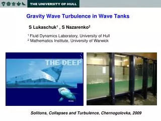
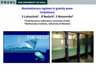
S Lukaschuk 1 , R Bedard 1 , S Nazarenko 2. 1 Fluid Dynamics Laboratory, University of Hull 2 Mathematics Institute, University of Warwick. Nonstationary regimes in gravity wave turbulence. Experiment. 8-panel Wave Generator. C 2. CCD. M. Laser. C 1.

E N D
S Lukaschuk1 , R Bedard1, S Nazarenko2 1Fluid Dynamics Laboratory, University of Hull 2 Mathematics Institute, University of Warwick Nonstationary regimes in gravity wave turbulence
Experiment 8-panel Wave Generator C2 CCD M Laser C1 Horizontal size: 8 x 12 m, water depth: up to 1 m
Theoretical predictions for spectra of stationary surface gravity waves • Weak turbulence theory (Zakharov, 1966 ) • Breaking waves (Phillips ,1958) sharp wave crests strong nonlinearity 2K. Breaking waves (Kuznetsov , 2004) slope breaks occurs in 1D lines wave crests are propagating with a preserved shape • Finite size effects (Zakharov 2005; Nazarenko et al 2006)
Set of experimental data Images: R S D D D One-point measurements 0 30 60 100 t, min
t-domain, rise filtered elevation Characteristic time
k-domain, Rise, small amplitudes(frozen turbulence) F1: 5 m-1 F2: 10 m-1 F3: 80 m-1 F4: 160 m-1 F5: 320 m-1
k-domain, Rise, medium amplitudes Breaking waves Front propagation F1: 5 m-1 F2: 10 m-1 F3: 80 m-1 F4: 160 m-1 F5: 320 m-1
k-domain, Rise, high amplitudes F1: 5 m-1 F2: 10 m-1 F3: 80 m-1 F4: 160 m-1 F5: 320 m-1
k-domain, Stationary, low & high amplitudes F1: 5 m-1 F2: 10 m-1 F3: 80 m-1 F4: 160 m-1 F5: 320 m-1
Decay characteristics estimates WT decay: Decay due to wall friction: Crossover amplitude:
-domain, decay of the main peak (~1 Hz)back wall 0 and 30 deg
t-domain, decay elevation RMS (t) Filter 4-7Hz
Conclusions • At the developing stage our experiment shows front propagation of turbulent energy along the k-spectra towards high k. In addition to this we observed a instantaneous injection of spectral energy into high k’s due to breaking events • At the late decay stage wave turbulent energy decreases exponentially in our case of an essentially small size flume, which due to significant contribution of wall friction • Finite size effects are responsible for non-monotonic decay of the wave spectrum tail. This effect is much more strong for “underdeveloped” turbulent regimes and not such significant for the case were initial state is characterized by a wide spectrum • Wave turbulence comprises a mixture of smooth chaotic waves and breaks which interact and influence each other • This influence were observed in our experiment as propagation of spectral humps down and up along the k-spectrum,