
Competitive Industries: A Study on Tipping in the Dishwashing Sector
E N D
Presentation Transcript
Introduction • BREAD encourages tipping for kitchen staff. • Impact of achieving goal: • In the short-run life will be better for dishwashers. • In the long-run, wages will decrease by full amount of tips so dishwasher take-home pay is not increased. • Chapter investigates: • Why wages are bid down by tips. • Who benefits from tipping? • Key point: dishwashing is a competitive industry.
Section 7.1 The competitive firm
Competitive Firm • A firm is perfectly competitive if it can sell any quantity it wants at the going market price. • A farm is a good example. • Generally firms with small market share and room to grow. • Firms with large market shares normally have to reduce prices to attract more customers. • Horizontal demand curve. • Products are interchangeable and buyers have many options.
Revenue Total Revenue = Price x Quantity For any competitive firm, marginal revenue = price Firm’s marginal revenue curve is flat at the going market price Demand curve for the product is also flat at the going market price
Firm’s Supply Decision • Produce good until MR = MC • Competitive firm produces a quantity where P = MC • Note: P ≡ MR • Supply curve • MC and supply are inverse functions • Supply curve looks like upward sloping portion of MC curve as long as MC curve upward sloping • SR and LR supply curves exist for the firm
Shutdowns and Exits • Does the producer want to produce the good? • Two distinctions • Shutdown: firm stops producing the good but still pays fixed costs • Exit: firm leaves the industry entirely and no longer faces any costs • Firms, in SR, can shutdown but not exit • Remains operational if P > AVC • In LR, can exit
Shutdowns • Shutdown occurs when firm stops producing. • Fixed costs continue for firms in shutdown. • Exit occurs when firm leaves an industry entirely. • No costs are incurred for firms that exit. • In the short run firms can shutdown, not exit. • Should not if Total Revenue > Variable Costs. • Firms continue to operate if, at profit maximizing quantity price of output exceeds average variable cost. • In the long run firms can exit.
Short-Run Supply Curve • When price falls below average variable cost, firm shuts down and produces nothing. • Supply curve is identical to the part of the marginal cost curve that lies above average variable cost curve. • Elasticity of Supply: • Percentage change in quantity supplied resulting from a 1% increase in price. • Positive because a price increase increases supply. • Given two curves through same point, flatter one has the higher elasticity.
Section 7.2 The competitive industry in the short run
Competitive Industry in the SR • All firms in industry competitive • SR is period of time in which no firm can enter or exit the industry • Number of firms cannot change • LR is period of time in which any firm can enter or leave the industry • Industry’s SR supply curve • Sum of SR individual firm supply curves • More elastic than individual supply curves
Supply, Demand, and Equilibrium • Each firm operates where supply meets demand • Industry equilibrium consequence of optimizing behavior on part of individuals and firms • Intersecting industry wide supply and industry wide demand
Competitive Equilibrium • Industry faces a downward-sloping demand curve. • Firms produces where supply (or marginal cost) curve crosses the horizontal line at the “going market price”. • Increase in fixed cost: • Marginal cost is unchanged so supply curve is unchanged. • Both price and quantity stay the same.
Competitive Equilibrium • Increase in variable cost: • Marginal costs rise and shift the supply curve leftward. • Higher market equilibrium price. • Industry output falls but firm’s output could go up or down. • Increase in industry demand: • Increase in firm’s output.
Change in Fixed Cost • Increase in FC • Price and quantity remain unchanged
Change in Variable Cost • Increase in VC • Raises firms MC curve • Causes some firms to shutdown • Higher market equilibrium price • Firm’s output could go up or down
Change in Industry Demand • Increase in industry demand • Higher market equilibrium price • Increase in firm’s output
Industry’s Costs Total cost are minimized when marginal cost is the same at every firm. In competitive equilibrium, every firm chooses to produce a quantity at which price = marginal cost. The equilibrium quantity is automatically produced at the lowest possible total cost.
Section 7.3 The competitive firm in the long run
Competitive Firm in the LR • Some short- run fixed costs become variable costs in the long run. • Firms can enter and exit in the long run. • The long-run supply curve is identical to the long-run marginal cost curve. • More elastic than the short-run supply curve.
Profit and the Exit Decision • Profit = TR – TC • Costs includes all foregone opportunities • SR versus LR supply response • Firm LR supply curve more elastic than SR supply curve • Shuts down if price of output falls below average variable cost • Exits if price of output falls below average cost
LRMC and Supply • Firms operate where P = LRMC • Remain in industry, LR supply curve identical to LRMC curve • Exit decision is made at the point P=AC (note that there is no more fixed cost in the LR)
Section 7.4 The competitive industry in the long run
Competitive Industry in the LR • Firms wishing to enter or exit the market do so in the LR, flatting out the LR supply curve • So unlike the case in the SR, the LR supply curve is a horizontal line. • Important assumption: all firms are identical in costs • Break-even price plays an important role here (1) all firms produce at the break-even price; (2) it determines the level of LR supply curve
Break-even • The price at which a seller earns zero profit. • Occurs where marginal and average cost curves cross. • In a constant-cost industry, the long-run industry supply curve is flat at the level of break-even. • Shifts every time the break-even price changes. • In the long-run, both fixed and variable costs matter. • Market price is determined by the intersection of the industry-wide supply and demand curves. • Firm faces flat demand curve at going market price.
Zero Profit Condition • Economic versus accounting profit • Accounting profit refers to total revenue minus total financial cost • Economic profit refers to accounting profit minus the value of the best foregone opportunity
Industry’s LR Supply Curve • All firms identical • Industry supply curve flat at the break-even price • Break-even price and the LR supply • Break-even price (P = AC) at which a seller earns zero profit • LR supply curve identical with part of firm’s LRMC curve lying above LRAC curve
Flat LR Supply Curve • Flatness based on entry and exit • P < AC, all firms exit • P > AC, unlimited number of firms enter • LR zero profit equilibrium almost never reached • Demand and cost curves shift so often that entry and exit never settles down • Approximation to the truth
Equilibrium • LR same as SR between firm and industry • Market price determined by intersection of industrywide demand and supply • Firms face flat demand curves at market price • Analysis of changes to equilibrium • Changes in FC • Changes in VC • Changes in demand
Application: Government as a Supplier • In the short-run, a government policy to build and operate an apartment complex increases available housing. • Equilibrium price falls. • In the long-run, supply curve does not shift. • Determined by break-even price. • Price of housing returns to break-even price. • Quantity provided returns to break-even quantity: • Number of privately owned apartments withdrawn from the market equals number of apartments built by government.
Relaxing the Assumptions • Assumption 1: All firms are identical, have identical cost curves • True in industries that do not require unusual skills • Assumption 2: Cost curves do not change as industry expands or contracts • True in industries not large enough to affect input prices • Without these assumptions, all firms do not have the same break-even price
Constant Cost • Constant cost industry • Satisfies the 2 assumptions