Boundary conditions
Boundary conditions. The external surface of the solid model need to be surround by proper boundary conditions The sound sources (loudspeakers) were modeled as areas where the normal acceleration is known as a function of frequency

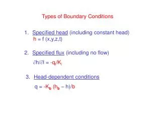
Boundary conditions
E N D
Presentation Transcript
Boundary conditions • The external surface of the solid model need to be surround by proper boundary conditions • The sound sources (loudspeakers) were modeled as areas where the normal acceleration is known as a function of frequency • The internal surfaces of the car are modeled as sourfaces of known complex acoustical impedence as a function of frequency • Some surfaces were modeled as rigid walls (glass, steel parts not covered by sound absorbing materials) • The values of acceleration and impedance were measured “in situ” thanks to novel hardware and software tools
Reference measurements in the car Hardware: PC and audio interface Edirol FA-101 Firewire sound card: 10 in / 10 out 24 bit, 192 kHz ASIO and WMA
Reference measurements in the car Software Aurora Plugins
Measurement process • The desidered result is the linear impulse response of the acoustic propagation h(t). It can be recovered by knowing the test signal x(t) and the measured system output y(t). It is necessary to exclude the effect of the not-linear part K and of the background noise n(t).
Test signal: Log Sine Sweep x(t) is a sine signal, which frequency is varied exponentially with time, starting at f1 and ending at f2.
Deconvolution of Log Sine Sweep The “time reversal mirror” technique is employed: the system’s impulse response is obtained by convolving the measured signal y(t) with the time-reversal of the test signal x(-t). As the log sine sweep does not have a “white” spectrum, proper equalization is required Test Signal x(t) Inverse Filter z(t)
Measured signal - y(t) • The not-linear behaviour of the loudspeaker causes many harmonics to appear
Inverse Filter – z(t) The deconvolution of the IR is obtained convolving the measured signal y(t) with the inverse filter z(t) [equalized, time-reversed x(t)]
1° 2° 3° 5° Result of the deconvolution The last impulse response is the linear one, the preceding are the harmonics distortion products of various orders
In-situ measurement of the acoustical properties • The measurement of the acoustical impedance is performed employing a Microflown pressure-velocity probe
In-situ measurement of the acoustical properties • The probe needs to be calibrated for proper gain and phase matching at low frequency Calibration over a reflecting surface Free-Field calibration
In-situ measurement of the acoustical properties • A specific software (Aurora plugin) has been developed for speeding up both calibration and measurement of the acoustical properties with the new pressure-velocity probe technique Input parameters Results