Understanding Lagrangian Boundary Conditions in Simulation Modeling
160 likes | 302 Vues
This chapter covers the fundamentals of Lagrangian boundary conditions in simulation modeling, focusing on concepts such as single point constraints (SPCn), enforced velocities, rigid walls, and tied connections. It explains the implementation of constraints to prevent motion in specific directions, model rotational conditions, and define enforced motions with respect to local coordinate systems. The chapter also dives into rigid body elements, the definition of connections between different mesh types, and how these concepts apply to realistic simulations of physical phenomena.

Understanding Lagrangian Boundary Conditions in Simulation Modeling
E N D
Presentation Transcript
CONTENTS • Single Point Constraints - SPCn • Enforced Velocities - FORCE/MOMENT • Rigid Walls - WALL • Tied Connections - RCONN • Rigid Body Elements • RBE2 • KJOIN • BJOIN
Single Point Constraint - SPC Prevents a point moving in a particular direction Must be initialized in the Case Control section: SPC = SID Any SPCn entries not selected in case control are ignored The displacement coordinate system of the constrained gridpoint determines the direction that the constraint is applied in Can be used to model boundary conditions and planes of symmetryAny component in grid coordinate system can be constrained Components in a grid coordinate system are referred by digits 1 to 6. Any combination is possible, e.g. 23,156 SPC=100 BEGIN BULK . . . SPC, 100, 27, 123 SPC1, 100, 156, 19, THRU, 28
Rotational Boundary Condition - SPC2 Used to model rotational boundary conditions on gridpoints Must be selected in Case Control SPC = SID
SINGLE POINT CONSTRAINT IN LOCAL COODINATES - SPC3 Used to define a single point constraint in a local coordinate system or a cascade of two local coordinate systems Must be selected in Case Control SPC = SID
Prescribes the motion of grid points Force of pressure loading - TYPE = 2 in TLOAD1 definitionMust be selected in Case ControlAny loading (TLOADn entry) not selected in Case Control is ignoredEnforced motion can be prescribed in a local coordinate system. ENFORCED MOTION
Specified points can have their velocity set Velocity - TYPE = 2 in TLOAD1 definitionTLOAD1, 100, 110, , 2, 120DAREA defines magnitude of translational or angular velocity per DOFFORCE defines magnitude and direction of translational velocityMOMENT defines magnitude and direction of angular velocityVelocity can vary arbitrarily with timeThe TABLED1 entry gives the variation of velocityTLOAD = 100 BEGIN BULK ... TLOAD1, 100, 110, , 2, 120 TABLED1, 120,,,,,,,, + +, 0.0, 0.0, 1.0, 1.0, ENDT FORCE, 110, 27, , -6.0, , 1.0 ENFORCED GRID POINT MOTION
FORCE in CORDXXXIf on a FORCE entry a CID is referenced, the enforced motion is processed in a local coordinate systemFORCE, 110, 27, 2 , -6.0, , 1.0 ENFORCED MOTION
RIGID WALLS - WALL • Models a rigid plane which specified ”slave” points can not penetrate • Used to model hard, undeformable target • Define a point on the wall and a vector perpendicular to it, pointing towards the model • Two kinds of contact: • PENALTY Method: Allowed penetration Force increases as nodes penetrate deeperCan have friction • KINEMATIC MethodNodes are put back on the SurfaceImpuls is applied to NodesCan not have friction WALL, 101, 0.0, 0.0, 0.0, 0.0, 0.0, 1.0, 102,+ +,PENALTY,0.2 SET1, 102, 1, THRU, 1999
TIED CONNECTIONS • Two meshes with different coarseness are permanently tied together during the analysis • Allows beam, shell and solid meshes to be tied together without the need for coinciding grid point locations • Possible gaps between the meshes can be requested to be closed • Not recommended in areas where stress peaks or failure is expected • Three types of tied connections: • • Two surfaces tied together • • Grid points tied to a surface • • Shell edge tied to a shell surface
TWO SURFACE TIED TOGETHER (RCONN) • Two surfaces are permanently tied together during the analysis • Master surface : always attached to the coarse mesh • Slave surface : always attached to the finer mesh • Lumping forces and velocities according to shape functions • Forces : slave points master points • Velocities : master points slave points • Example: Two solids are tied together along their common surface 7 and 8 • RCONN, 1, SURF, SURF, 7, 8
GRID POINTS TIED TO A SURFACE (RCONN) • Individual grid points are tied to a surface • Slave surface type is GRID and OPTION must be set to NORMALMaster surface must be defined as a set of segments • Only the translational degrees of freedom are tied • Example: The node 1 to 10 of a beam mesh are tied to the shell surface 7 • RCONN, 1, GRID, SURF, 3, 7, NORMAL • SET1, 3, 1, THRU, 10
SHELL EDGE TIED TO A SHELL SURFACE • Connects beams or shell-edges to shell elements • Slave surface type is GRID and OPTION must be set to SHELLMaster surface must be defined as a set of segments • Translational and rotational degrees of freedom are tied. • Example: The edge grid points 1 to 10 of a shell mesh are tied to the shell surface number 7 • RCONN, 1, GRID, SURF, 3, 7, SHELL • SET1, 3, 1, THRU, 10
RIGID BODY ELEMENTS (RBE2) Defines a set of grid points that form a rigid body This entry allows particular degrees of freedom of a set of grid points to be tied together so that they always move the same amount Used to model spotwelds, but elements can not fail Example: Nodes 1 to 28 will have the same displacement in x and z-direction as node 55 RBE,12,55,13,1,THRU,28 Instead of defining tied components, it is also possible to use the FULLRIG option This causes the set of grid points to behave like a single rigid body elementThe name of the RBE2 will become FR<number> Example: Nodes 1 to 28 and 55 will behave like a rigid body The name will be FR12 RBE,12,55,FULLRIG,1,THRU,28
R1 R2 SHELLS C R3 Rotation at C follows from the motion of the system Ri SOLIDS KINEMATIC JOIN (KJOIN) Shell to solid grid point connection Joins shell to solid elements by applying kinematic conditions to the shell grid points A normal JOIN would result in a hinge connection in which only the translational DOFs are coupled Solves the closure problem for the different DOF of shell and solid elements Constitutes stiff connection between shells and solids Stiffness of join is user defined Example: Kjoin between solid nodes 30, 40 and 50 and shell nodes 32, 42 and 52 All nodes within a tolerance of 1e-5 are connected KJOIN, 2, 333,1e-5,, 0.5 SET1, 333, 30, 32, 40, 42, 50, 52
BREAKABLE JOIN (BJOIN) • Defines a breakable join between shell or beam grid points • Joins shell or beam grid points and allows for the break of the join when a failure criterion is satisfied • Failure models : • Constant Force or Moment • Components Failure • Spotweld like behavior • User defined • Breakable join can have offset (spotweld modeling) • Example: Breakable join that fails after 1.e6 is reached All nodes within a tolerance of 1e-4 are connected • BJOIN, 1, 333, 1.E-4, FOMO, 1.E6 • SET1, 333, 31, THRU, 2000