Download
1 / 47
510 likes | 635 Vues
This chapter delves into the application of boundary conditions using Chebyshev nodes and derivative matrices in MATLAB. It presents two main methods: establishing boundary conditions through unique polynomial interpolants and adding equations to enforce these conditions. It also addresses the behavior of Chebyshev differential matrices and their eigenvalues. Diverse examples include linear and nonlinear boundary value problems, such as the Allen-Cahn equation, with detailed solutions demonstrating effective strategies for handling boundary conditions in computational contexts.

E N D
Chapter 13 More about Boundary conditions Speaker: Lung-Sheng Chien Book: Lloyd N. Trefethen, Spectral Methods in MATLAB
Preliminary: Chebyshev node and diff. matrix [1] Consider Chebyshev node on for Uniform division in arc Even case: Odd case:
Preliminary: Chebyshev node and diff. matrix [2] Given Chebyshev nodes and corresponding function value We can construct a unique polynomial of degree , called is a basis. where differential matrix is expressed as for for where with identity Second derivative matrix is
Preliminary: Chebyshev node and diff. matrix [3] and Let be the unique polynomial of degree with define and for , then impose B.C. ,that is, We abbreviate In order to keep solvability, we neglect ,that is, zero neglect zero neglect Similarly, we also modify differential matrix as
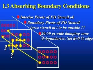
Asymptotic behavior of spectrum of Chebyshev diff. matrix In chapter 10, we have showed that spectrum of Chebyshev differential matrix (second order) approximates with eigenmode 1 Eigenvalue of is negative (real number) and Large eigenmode of does not approximate to 2 Since ppw is too small such that resolution is not enough Mode N is spurious and localized near boundaries
Preliminary: DFT [1] Given a set of data point with is even, Then DFT formula for for for Definition: band-limit interpolant of , is periodic sinc function If we write , then Also derivative is according to
Preliminary: DFT [2] , we have Direct computation of derivative of Example: is a Toeplitz matrix. Second derivative is
Preliminary: DFT [3] For second derivative operation second diff. matrix is explicitly defined by using Toeplitz matrix (command in MATLAB) Symmetry property:
Preliminary: DFT [4] is corresponding to eigenvector Eigenvalue of Fourier differentiation matrix has multiplicity 2 and for and when and , we have
How to deal with boundary conditions • Method I: Restrict attention to interpolants that satisfy the boundary conditions. Example: chapter 7. Boundary value problems Linear ODE: Nonlinear ODE: Eigenvalue problem: Poisson equation: Helmholtz equation: • Method II: Do not restrict the interpolants, but add additional equations to enforce the boundary condition.
Recall linear ODE in chapter 7 with exact solution Chebyshev nodes: be unique polynomial of degree with and Let 1 for Method I Set for 2 zero neglect zero neglect
Inhomogeneous boundary data [1] Method I and be unique polynomial of degree with Let 1 for Set for 2 1 neglect zero neglect or say
Inhomogeneous boundary data [2] Method of homogenization , decompose , then satisfies which can be solved by method I Solution under N = 16 method I directly method of homogenization method I is good even for inhomogeneous boundary data exact solution
Mixed type B.C. [1] Method I and be unique polynomial of degree with Let 1 for How to do? Set for 2 Method II and be unique polynomial of degree with Let 1 for easy to do Set for 2 zero neglect neglect
Mixed type B.C. [2] , we add one more constraint (equation) Set 3 zero zero Active variable with governing equation from interior point from Neumann condition In general, replace by since the method works for
Mixed type B.C. [3] exact solution Solution under N = 16
Allen-Cahn (bistable equation) [1] Nonlinear reaction-diffusion equation: where is a parameter 1 This equation has three constant steady state, , equilibrium occurs at zero forcing ) ( consider ODE is unstable and is attractor. 2 is Logistic equation. for
Allen-Cahn (bistable equation) [2] for , separated by interfaces Solution tends to exhibit flat areas close to 3 That may coalesce or vanish on a long time scale, called metastability. interface boundary value:
Allen-Cahn : example 1 [1] with parameter and initial condition Method I and be unique polynomial of degree with Let 1 for Set for 2 1 neglect -1 neglect or say
Allen-Cahn : example 1 [2] Temporal discretization: forward Euler with CFL condition ( eigenvalue of is negative (real number) and ) One can simplify above equation by using equilibrium of at boundary point.
Allen-Cahn : example 1 [3] with parameter and initial condition Solution under N = 20 boundary value: interface Metastability up to followed by rapid transition to a solution with just one interface.
Allen-Cahn : example 2 [1] with parameter and initial condition Method I be unique polynomial of degree with Let 1 and for Set for 2 Second, set
Allen-Cahn : example 2 [2] However we cannot simplify as following form is NOT an equilibrium. since Method II for be unique polynomial of degree with Let 1 2 Set for 3 Neglect computed from 2 , and reset
Allen-Cahn : example 2 [3] Step 1: Step 2: Solution under N = 20,method II Final interface is moved from to and transients vanish earlier at instead of and
Allen-Cahn : example 2 [4] graph concave up ? Threshold is In fact we can estimate trend of transient at point and , then but
Laplace equation [1] subject to B.C. boundary data is continuous for be unique polynomial, Let 1 Method I for (interior point) and for Set 2 Briefly speaking, method I take active variables as However method 1 is not intuitive to write down linear system if we choose Kronecker-product
Laplace equation [2] Method II for be unique polynomial, Let 1 (all points) (interior points) for Set 2 Additional constraints (equations) for boundary condition. 3 for method II take active variables as Technical problem: 1. How to order the active variables 2. How to build up linear system (matrix) (including second derivative and additional equation) 3. How to write down right hand side vector
Laplace equation : order active variable [3] MATLAB use column-major, so we index active variable by column-major and 31 25 19 13 7 1 32 26 20 14 8 2 33 27 21 15 9 3 column-major 34 28 22 16 10 4 35 29 23 17 11 5 18 36 30 24 12 6
Laplace equation : find boundary point [6] b is index set of boundary points, if we write down equations according to index of active variables, then we can use index setb to modify the linear system. Chebyshev differentiation matrix: (second order)
Laplace equation : construct matrix [7] (interior points) for Set 2 Definition: Kronecker product is defined by
Laplace equation : construct matrix [8] Additional constraints (equations) for boundary condition. 3 for on boundary points by We need to replace equation of Index of boundary points for such that (boundary point) where four corner points each edge has N-1 points
Laplace equation : right hand side vector [9] Boundary data: identify 31 25 19 13 7 1 32 26 20 14 8 2 33 27 21 15 9 3 34 28 22 16 10 4 35 29 23 17 11 5 18 36 30 24 12 6
Laplace equation : right hand side vector [10] Boundary data: identify 31 25 19 13 7 1 32 26 20 14 8 2 33 27 21 15 9 3 34 28 22 16 10 4 35 29 23 17 11 5 18 36 30 24 12 6
Laplace equation : results [11] Solution under N = 5,method II Solution under N = 24,method II
Wave equation [1] subject to B.C. Separation of variables leads to Fourier discretization in x Periodic B.C. in x-coordinate 1 2 Chebyshev discretization in y, we must deal with Neumann B.C. 3 Leap-frog formula in time Leap-frog eigenvalue of (chebyshev diff. matrix) is negative and eigenvalue of (Fourier diff. matrix) is eigenvalue of (Fourier diff. matrix) is negative and Hence stability requirement of is ( author chooses )
Wave equation [2] Fourier discretization in x Periodic B.C. in x-coordinate 1 2 Chebyshev discretization in y Method II be unique polynomial of degree with Let for 1 Set for 2 3 replace computed from 2 by Neumann B.C. Chebyshev diff. matrix
Wave equation: order active variable [3] 1 7 13 19 25 31 2 14 20 26 32 8 9 21 27 33 column-major 3 15 4 22 28 10 16 34 23 29 35 5 11 17 6 18 24 30 36 12 In this example, we don’t arrange as vector but keep in 2-dimensional form say , the same arrangement of xx and yy generated by meshgrid(x,y)
Wave equation: action of Chebyshev operator [4] Chebyshev 2nd diff. matrix 1 7 13 19 25 31 2 14 20 26 32 8 9 21 27 33 3 15 4 22 28 10 16 34 23 29 35 5 11 17 6 18 24 30 36 12 index ( i,j ) is logical index according to index of ordinates x, y
Wave equation: action of Fourier operator [5] Fourier 2nd diff. matrix 6 5 4 3 2 1 12 11 10 9 8 7 18 17 16 15 14 13 24 23 22 21 20 19 30 29 28 27 26 25 36 35 34 33 32 31 Take transpose
Wave equation: action of operator [6] , then operator for Laplacian is Let active variable be Combine with Leap-frog formula in time where initial condition is Gaussian pilse traveling rightward at speed 1 Question: how to match Neumann boundary condition
Wave equation: Neumann B.C. in y-coordinate [7] 3 replace computed from 2 by Neumann B.C. We require or say for
Wave equation: Neumann B.C. in y-coordinate [8] or say where written as Procedure of wave equation simulation Given Step 1: time evolution by Leap-frog Step 2: correct boundary data where
Wave equation: result [9] Solution under , method II Theoretical optimal value is (see exercise 13.4)
Exercise 13.2 [1] The lifetime of metastable state depends strongly on the diffusion constant The value of t at which first becomes monotonic in x. with parameter and initial condition what is graph of 1 Asymptotic behavior of 2 as
Exercise 13.2 [2] • Resolution is adaptive and • Monotone under tolerance