GWAS and R
GWAS and R. Nathan Tintle, Dordt College Jason Westra, Dordt College and Trinity Christian HS. History of group. 2005-2011. Michigan (Hope College/ Univ of Michigan) Statistical genetics methods research Undergraduate research assistants (summer and academic year)

GWAS and R
E N D
Presentation Transcript
GWAS and R Nathan Tintle, Dordt CollegeJason Westra, Dordt College and Trinity Christian HS
History of group • 2005-2011. Michigan (Hope College/ Univ of Michigan) • Statistical genetics methods research • Undergraduate research assistants (summer and academic year) • Funding via NIH, NSF, etc. • Lots of Monte Carlo simulation to validate methods proposals; Little real data analysis • Techniques: Arrays, simulation of large datasets; function (object) programming; loops and conditionals; exploratory data analysis • Statistics education • Randomization and simulation in the first course (http://math.hope.edu/isi). Not using R, but could!
History of group • Move towards applied problems • Use of large-scale genomic data to validate methods • Application of methods to real genetic data through growing applied science collaborations (e.g., Sanford, Umichigan, Utah State, Argonne National Labs, etc) • Growing pains • Different R challenges; computational needs; managing (opening, using) large datasets • Analysis quality and confidence (can’t confirm work via methods= simulation results)
Brief introduction to GWAS • Genome-wide association study • Attempt to associate genetic variation with phenotype changes • Examples: Differences in the genetic structure at a particular location in the genome increase the risk of a disease
Genetics primer • DNA—building block of life consists of long strands of nucleotide “base pairs” [bp, A-T or T-A or C-G or G-C] which contains the genetic blueprint for the individual • Human DNA is organized into 23 pairs of chromosomes (a continuous strand of DNA) • One chromosome in each pair is obtained from the mother, the other from the father
Genetics primer • Each person has a sequence of 3 billion A, C, T, G’s spread across the 23 chromosomes • …..AAATCTATCTGGTGACCCTCATG……… • Two copies of each • One from Mom and one from Dad
Genetics primer • Single Nucleotide Variants (SNVs) • - A single nucleotide difference between two individuals • Estimates are 10-30 million SNPs (SNVs with at least 1% population prevalence) • Rarer variation much more common SNP
Simplest version of the problem • Standard study design and analysis for traditional GWAS • Genotype the SNPs for a bunch of people with and without the disease • Compare each locus to see if a different genotype distribution was present in cases vs. controls
Challenges • Lots and lots of chi-squared tests (hundreds of thousands to millions of them!) • Identify the minor (typically risk increasing) allele (assign value 0,1,2) • Missing data, lack of hardy-weinberg equilibrium and other genotype QC • Outputs: p-values for each SNP, estimated effects sizes, contextual information (MAF, LD structure, chromosome/bp/gene, other bioinformatic info)
More complex versions of the problem • Extra correlation between subjects • Family based data in Framingham heart study • History of Framingham; data structure • Can’t just use regression/chi-squared tests anymore; more advanced statistical methods that model the correlation structure are needed
More complex versions of the problem • Accounting for covariates; quant response Genotype (SNP) Disease/Phenotype Diet; Ethnicity; other covariates
More complex versions of the problem • Fatty acid level = Genotype + Diet + Supplement + Age + Sex + more?? • Fitting multiple nested models
More complex versions of the problem • Biologically informed analyses • Aggregating by gene or pathway • Reduces multiple testing penalties • Generates more biologically plausible
More complex versions of the problem • Imputed SNPs • Genotypes not directly measured by ‘predicted’ • More complex file structures; different for different SNPs • More/different quality information
SNPS 500500 X 14400 Matrix 500500 X 1200 Matrix Pedigree file Fatty Acid Age, Sex Dietary Information .2 sec 27.7 hrs Minor/Major allele, Minor allele freq. Hardy-Weinberg Equilibrium Singletons Phenotypes 2800 X 70 Matrix Kinship Matrix 17500 X 17500 dsCMatrix Minor Allele Frequency 500500 X 2800 Matrix GWAS Function:(Fatty acid, phenotypes) Merge(minor allele frequency/phenotypes) Create a dynamic formula from the function call lmekin(formula, kinship matrix) List output from lmekin includes beta value Calculate pval from output list Save SNPid Beta Pval Minor Allele Frequency 50 Matrices 10000 X 2800 5.6 sec 777.78 hrs
Lessons Learned • Vector vs. Matrix • Vectors were 4 times faster. • PBS Job arrays • qsub –t 1-50 GWAS
Bottlenecks • Lmekin function • Each snp takes 5.6 seconds to run • 5.55 seconds for lmekin • 0.05 seconds for other processes • Cluster availability • Currently using 32 nodes • Increasing to 64 nodes would cut time in half.
Moving Forward • Real-time bioinformatics • 5 million SNPs • 10+ million SNPs in the next 12 to 18 months • Covariates • More of them • Different combinations • Different fatty acids • Fatty acid ratios • And the fun continues • Many GB worth of raw RNA-seq data uploaded from a collaborator over the last few days: pipelines for analysis and interpretation now needed!! • Potential upgrade to computational resources (parallel computer in Michigan) • GPUs vs. CPUs • RAM, “smarter” parallel processing to improve computational time • More nodes vs. More RAM vs. Increased processor speed