Download
1 / 48
480 likes | 746 Vues
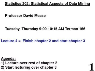
Statistics 202: Statistical Aspects of Data Mining Professor David Mease Tuesday, Thursday 9:00-10:15 AM Terman 156 Lecture 4 = Finish chapter 2 and start chapter 3 Agenda: 1) Lecture over rest of chapter 2 2) Start lecturing over chapter 3. Announcement:

E N D
Statistics 202: Statistical Aspects of Data Mining Professor David Mease Tuesday,Thursday 9:00-10:15AM Terman 156 Lecture 4 = Finish chapter 2 and start chapter 3 Agenda: 1) Lecture over rest of chapter 2 2) Start lecturing over chapter 3
Announcement: One of the TAs, Ya Xu (yax@stanford.edu), will hold office hours on Monday, July 9th from 1pm to 3pm to assist with last minute homework questions and any other questions. Her office is 237 Sequoia Hall.
Homework Assignment: Chapters 1 and 2 homework is due Tuesday 7/10 Either email to me (dmease@stanford.edu), bring it to class, or put it under my office door. SCPD students may use email or fax or mail. The assignment is posted at http://www.stats202.com/homework.html
Introduction to Data Mining by Tan, Steinbach, Kumar Chapter 2: Data
What is Data? • An attribute is a property or characteristic of an object • Examples: eye color of a person, temperature, etc. • Attribute is also known as variable, field, characteristic, or feature • A collection of attributes describe an object • Object is also known as record, point, case, sample, entity, instance, or observation Attributes Objects
Sampling (P.47) • Sampling involves using only a random subset of the data for analysis • Statisticians are interested in sampling because they often can not get all the data from a population of interest • Data miners are interested in sampling because sometimes using all the data they have is too slow and unnecessary
Sampling (P.47) • The key principle for effective sampling is the following: • using a sample will work almost as well as using the entire data sets, if the sample is representative • a sample is representative if it has approximately the same property (of interest) as the original set of data
Sampling (P.47) • The simple random sample is the most common and basic type of sample • In a simple random sample every item has the same probability of inclusion and every sample of the fixed size has the same probability of selection • It is the standard “names out of a hat” • It can be with replacement (=items can be chosen more than once) or without replacement (=items can be chosen only once) • More complex schemes exist (examples: stratified sampling, cluster sampling, Latin hypercube sampling)
Sampling in Excel: • The function rand() is useful. • But watch out, this is one of the worst random number generators out there. • To draw a sample in Excel without replacement, use rand() to make a new column of random numbers between 0 and 1. • Then, sort on this column and take the first n, where n is the desired sample size. • Sorting is done in Excel by selecting “Sort” from the “Data” menu
Sampling in R: • The function sample() is useful.
In class exercise #4: Explain how to use R to draw a sample of 10 observations with replacement from the first quantitative attribute in the data set www.stats202.com/stats202log.txt.
In class exercise #4: Explain how to use R to draw a sample of 10 observations with replacement from the first quantitative attribute in the data set www.stats202.com/stats202log.txt. Answer: > sam<-sample(seq(1,1922),10,replace=T) > my_sample<-data$V7[sam]
In class exercise #5: If you do the sampling in the previous exercise repeatedly, roughly how far is the mean of the sample from the mean of the whole column on average?
In class exercise #5: If you do the sampling in the previous exercise repeatedly, roughly how far is the mean of the sample from the mean of the whole column on average? Answer: about 26 > real_mean<-mean(data$V7) > store_diff<-rep(0,10000) > > for (k in 1:10000){ + sam<-sample(seq(1,1922),10,replace=T) + my_sample<-data$V7[sam] + store_diff[k]<-abs(mean(my_sample)-real_mean) + } > mean(store_diff) [1] 25.75126
In class exercise #6: If you change the sample size from 10 to 100, how does your answer to the previous question change?
In class exercise #6: If you change the sample size from 10 to 100, how does your answer to the previous question change? Answer: It becomes about 8.1 > real_mean<-mean(data$V7) > store_diff<-rep(0,10000) > > for (k in 1:10000){ + sam<-sample(seq(1,1922),100,replace=T) + my_sample<-data$V7[sam] + store_diff[k]<-abs(mean(my_sample)-real_mean) + } > mean(store_diff) [1] 8.126843
The square root sampling relationship: • When you take samples, the differences between the sample values and the value using the entire data set scale as the square root of the sample size for many statistics such as the mean. • For example, in the previous exercises we decreased our sampling error by a factor of the square root of 10 (=3.2) by increasing the sample size from 10 to 100 since 100/10=10. This can be observed by noting 26/8.1=3.2. • Note: It is only the sizes of the samples that matter, and not the size of the whole data set.
Sampling (P.47) • Sampling can be tricky or ineffective when the data has a more complex structure than simply independent observations. • For example, here is a “sample” of words from a song. Most of the information is lost. oops I did it again I played with your heart got lost in the game oh baby baby oops! ...you think I’m in love that I’m sent from above I’m not that innocent
Sampling (P.47) • Sampling can be tricky or ineffective when the data has a more complex structure than simply independent observations. • For example, here is a “sample” of words from a song. Most of the information is lost. oops I did it again I played with your heart got lost in the game oh baby baby oops! ...you think I’m in love that I’m sent from above I’m not that innocent
Introduction to Data Mining by Tan, Steinbach, Kumar Chapter 3: Exploring Data
Exploring Data • We can explore data visually (using tables or graphs) or numerically (using summary statistics) • Section 3.2 deals with summary statistics • Section 3.3 deals with visualization • We will begin with visualization • Note that many of the techniques you use to explore data are also useful for presenting data
Visualization • Page 105: “Data visualization is the display of information in a graphical or tabular format. Successful visualization requires that the data (information) be converted into a visual format so that the characteristics of the data and the relationships among data items or attributes can be analyzed or reported. The goal of visualization is the interpretation of the visualized information by a person and the formation of a mental model of the information.”
Example: Below are exam scores from a course I taught once. Describe this data. 192 160 183 136 162 165 181 188 150 163 192 164 184 189 183 181 188 191 190 184 171 177 125 192 149 188 154 151 159 141 171 153 169 168 168 157 160 190 166 150 Note, this data is at www.stats202.com/exam_scores.csv
The Histogram • Histogram (Page 111): “A plot that displays the distribution of values for attributes by dividing the possible values into bins and showing the number of objects that fall into each bin.” • Page 112 – “A Relative frequency histogram replaces the count by the relative frequency”. These are useful for comparing multiple groups of different sizes. • The corresponding table is often called the frequency distribution (or relative frequency distribution). • The function “hist” in R is useful.
In class exercise #7: Make a frequency histogram in R for the exam scores using bins of width 10 beginning at 120 and ending at 200.
In class exercise #7: Make a frequency histogram in R for the exam scores using bins of width 10 beginning at 120 and ending at 200. Answer: > exam_scores<- read.csv("exam_scores.csv",header=F) > hist(exam_scores[,1],breaks=seq(120,200,by=10), col="red", xlab="Exam Scores", ylab="Frequency", main="Exam Score Histogram")
In class exercise #7: Make a frequency histogram in R for the exam scores using bins of width 10 beginning at 120 and ending at 200. Answer:
The (Relative) Frequency Polygon • Sometimes it is more useful to display the information in a histogram using points connected by lines instead of solid bars. • Such a plot is called a (relative) frequency polygon. • This is not in the book. • The points are placed at the midpoints of the histogram bins and two extra bins with a count of zero are often included at either end for completeness.
In class exercise #8: Make a frequency polygon in R for the exam scores using bins of width 10 beginning at 120 and ending at 200.
In class exercise #8: Make a frequency polygon in R for the exam scores using bins of width 10 beginning at 120 and ending at 200. Answer: > my_hist<-hist(exam_scores[,1], breaks=seq(120,200,by=10),plot=FALSE) > counts<-my_hist$counts > breaks<-my_hist$breaks > plot(c(115,breaks+5), c(0,counts,0), pch=19, xlab="Exam Scores", ylab="Frequency",main="Frequency Polygon") > lines(c(115,breaks+5),c(0,counts,0))
In class exercise #8: Make a frequency polygon in R for the exam scores using bins of width 10 beginning at 120 and ending at 200. Answer:
The Empirical Cumulative Distribution Function (Page 115) • “A cumulative distribution function (CDF) shows the probability that a point is less than a value.” • “For each observed value, an empirical cumulative distribution function (ECDF) shows the fraction of points that are less than this value.” (Page 116) • A plot of the ECDF is sometimes called an ogive. • The function “ecdf” in R is useful. The plotting features are poorly documented in the help(ecdf) but many examples are given.
In class exercise #9: Make a plot of the ECDF for the exam scores using the function “ecdf” in R.
In class exercise #9: Make a plot of the ECDF for the exam scores using the function “ecdf” in R. Answer: > plot(ecdf(exam_scores[,1]), verticals= TRUE, do.p=FALSE, main="ECDF for Exam Scores", xlab="Exam Scores", ylab="Cumulative Percent")
In class exercise #9: Make a plot of the ECDF for the exam scores using the function “ecdf” in R. Answer:
Comparing Multiple Distributions • If there is a second exam also scored out of 200 points, how will I compare the distribution of these scores to the previous exam scores? • 187 143 180 100 180 • 159 162 146 159 173 • 151 165 184 170 176 • 163 185 175 171 163 • 170 102 184 181 145 • 154 110 165 140 153 • 182 154 150 152 185 • 140 132 • Note, this data is at www.stats202.com/more_exam_scores.csv
Comparing Multiple Distributions • Histograms can be used, but only if they are Relative Frequency Histograms. • Relative Frequency Polygons are even better. You can use a different color/type line for each group and add a legend. • Plots of the ECDF are often even more useful, since they can compare all the percentiles simultaneously. These can also use different color/type lines for each group with a legend.
In class exercise #10: Plot the relative frequency polygons for both the first and second exams on the same graph. Provide a legend.
In class exercise #10: Plot the relative frequency polygons for both the first and second exams on the same graph. Provide a legend. Answer: > more_exam_scores<- read.csv("more_exam_scores.csv",header=F) > my_new_hist<- hist(more_exam_scores[,1], breaks=seq(100,200,by=10),plot=FALSE) > new_counts<-my_new_hist$counts > new_breaks<-my_new_hist$breaks > plot(c(95,new_breaks+5),c(0,new_counts/37,0), pch=19,xlab="Exam Scores", ylab="Relative Frequency",main="Relative Frequency Polygons",ylim=c(0,.30)) > lines(c(95,new_breaks+5),c(0,new_counts/37,0), lty=2)
In class exercise #10: Plot the relative frequency polygons for both the first and second exams on the same graph. Provide a legend. Answer (Continued): > points(c(115,breaks+5),c(0,counts/40,0), col="blue",pch=19) > lines(c(115,breaks+5),c(0,counts/40,0), col="blue",lty=1) > legend(110,.25,c("Exam 1","Exam 2"), col=c("black","blue"),lty=c(2,1),pch=19)
In class exercise #10: Plot the relative frequency polygons for both the first and second exams on the same graph. Provide a legend. Answer (Continued):
In class exercise #11: Plot the ecdf for both the first and second exams on the same graph. Provide a legend.
In class exercise #11: Plot the ecdf for both the first and second exams on the same graph. Provide a legend. Answer: > plot(ecdf(exam_scores[,1]), verticals= TRUE,do.p = FALSE, main ="ECDF for Exam Scores", xlab="Exam Scores", ylab="Cumulative Percent", xlim=c(100,200)) > lines(ecdf(more_exam_scores[,1]), verticals= TRUE,do.p = FALSE, col.h="red",col.v="red",lwd=4) > legend(110,.6,c("Exam 1","Exam 2"), col=c("black","red"),lwd=c(1,4))
In class exercise #11: Plot the ecdf for both the first and second exams on the same graph. Provide a legend. Answer:
In class exercise #12: Based on the plot of the ECDF for both the first and second exams from the previous exercise, which exam has lower scores in general? How can you tell from the plot?