Introduction to the Hankel -based model order reduction for linear systems
220 likes | 632 Vues
Introduction to the Hankel -based model order reduction for linear systems. D.Vasilyev. Massachusetts Institute of Technology, 2004. State-space description. MIMO LTI CT dynamical system :. Here we assume a system to be stable, i.e matrix A is Hurwitz. Model order reduction problem.

Introduction to the Hankel -based model order reduction for linear systems
E N D
Presentation Transcript
Introduction to the Hankel -based model order reduction for linear systems D.Vasilyev Massachusetts Institute of Technology, 2004
State-space description MIMO LTI CT dynamical system: Here we assume a system to be stable, i.e matrix A is Hurwitz.
Model order reduction problem y(t) u(t) e(t) G(s) (original) + - Gr(s) (reduced) yr(t) Problem: find a dynamical system Gr(s) of a smaller degree q (McMillan degree – size of a minimal realization), such that the error of approximation e is “small” over all inputs! Question: small in what sense??
Signals/system norms L2 – space of square-summable functions with 2- norm, or energy: u t LTI system, as a linear operator on this space, has an induced 2-norm (maximum energy amplification, or L2 gain), which equals H-infinity-norm of a system’s transfer function: Now we know how to state our problem!
Model order reduction problem y(t) u(t) e(t) G(s) (original) + - Gr(s) (reduced) yr(t) Problem formulation: find Gr(s) of a smaller degree that minimizes Unfortunately, we cannot solve this problem Instead, we use another system norm.
Hankel operator Hankel operator u y LTI SYSTEM t t Past input (u(t>0)=0) Future output X (state) • Hankel operator: • maps past inputs to future system outputs • ignores any system response before time 0. • Has finite rank (connection only by the state at t=0) • As an operator on L2 it has an induced norm (energy amplification)!
Hankel optimal MOR y(t) u(t) e(t) G(s) (original) + - Gr(s) (reduced) yr(t) Problem formulation: find Gr(s) of a smaller degree that minimizes (Hankel norm of an error) This problem has been solved and explicit algorithm is given for state-space LTI systems in Glover[84].
Hankel operator Controllability/observability u y LTI SYSTEM t t Past input Future output X (state) P (controllability) Which states are easier to reach? Q (observability) Which states produces more output? Since we are interested in Hankel norm, we need to know how energy is transferred between input, state and output
Observability y X(0) Future output t How much energy in the output we shall observe if the system is released from some state x(0)? Observability Gramian Satisfies Lyapunov equation: ATQ +QA = -CTC Q is SPD iff system is observable
Controllability u Past input X(0) State t What is the minimal energy of input signal needed to drive system to the state x(0)? Controllability Gramian Satisfies Lyapunov equation: AP + PAT = -BBT P is SPD iff system is controllable
Side note about Lyapunov equations AP + PA′ = -R, R - hermitian This equation has a unique solution P=P′if and only if: Moreover, if R is SPD and A is Hurwitz, then P is SPD. Assume some LTI CT system: Lyapunov function: V(x)=x’Px >0 (reformulation of stability criterion)
Hankel operator Hankel singular values u y X (state) t t - This operator has finite rank (equal to degree of G). Hankel singular values are square roots of an eigenvalues of the product PQ - If we approximate this operator by different one with lower rank, we cannot do better in the Hankel norm than the first removed HSV: Amazingly, this bound is tight (Adamjan et al., 71)
Truncated balanced reduction Gramians are transformed with the change of basis as a quadratic forms: x → Tx, P → TPTT, Q → T-TQT-1 We can find a basis, in which both gramians are equal and diagonal. Such transformation is called balancing transformation. T = RTU Σ-1/2 P = RTR UΣ2UT = RQRT P = Q = diag(σ1, … , σn), σ1 ≥ … ≥ σn
Truncated balanced reduction-cont’d In the balanced realization we can perform truncation of the least observable and controllable modes! Truncated system (A11, B1, C1, D) will be stable (if σq ≠σq+1 , otherwise stable for almost all T) and have the following H-infinity error bound: “twice sum of a tail” rule
Truncated balanced reduction vs. Hankel optimal reduction For the balanced truncation procedure we have the following error bounds: TBR is not optimal in terms of the Hankel norm! For the Hankel optimal MOR the following bounds hold:
References: • Keith Glover, “All optimal Hankel-norm approximations of linear multivariable systems and their L-infinity error bounds”