Parallel Computation Architecture, Algorithm and Programming

1. Textbook Series for 21st Century Parallel ComputationArchitecture, Algorithm and Programming Professor Guoliang Chen Dept. Of Comp. Sci. & Tech. Univ. Of Sci.&Tech. Of China

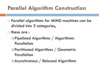
2. Chapter 1Architecture models of parallel computer Part I: Hardware basics for parallel computing • Browse the homepages of HPCC in USA. • A crossbar chip design for SP2 • Multistage crossbar network in Cray Y-MP • The structure of fat tree (the four-way fat tree implemented in CM-5)

3. A crossbar chip design for SP2 Part I: Hardware basics for parallel computing • Buffered wormhole routing is used • No conflict: 8 packet cells (called flits) pass through the 8x8 switch in every 40MHz cycle • hot-spot conflict: only one crosspoint will be enabled at a time • Central queue • Dual-port RAM, 1 read&1 write in a clock cycle • deserializes eight flits from FIFO into a chunk, then write it to the central queue in one cycle

4. Part I: Hardware basics for parallel computing Multistage crossbar network in Cray Y-MP • 4x4 and 8x8 crossbar switches and 1x8 de-multiplexors in three stages • supporting data streaming between 8 vector processors and 256 memory banks

5. The structure of multiway fat tree Part I: Hardware basics for parallel computing • Alleviate the bottleneck towards the root of a tree structure (Leiserson 1985) • the number of links increases when traversing from a leaf node toward the root • Each node has 4 child nodes and 2 or 4 parent nodes (shown in left figure)

6. Part I: Hardware basics for parallel computing Exercises (1) • In a two-way fat tree shown in Figure 1.33, each node has 2 parent nodes. If each oval in the figure is looked as a single node and the multi-edge between a pair of nodes is looked as one edge, then the fat tree can be looked as a binary tree. The question is, if we look each square but not the oval in the figure as a node, then what multilevel internet will it be when looked from the leaves to the root? • In a butterfly network shown in Fig. 1.37, N=(k+1)2k. Node degree=? Network Diameter=? And Bisection width=?

7. Exercises (2) Part I: Hardware basics for parallel computing • The Cedar multiprocessor at Illinois is built with a clustered Omega network as shown in the following figure. Four 8x4 crossbar switches are used in stage 1 and four 4x8 crossbar switched are used in stage 2. There are 32 processors and 32 memory modules, devided into four clusters with eight processors per cluster • Figure out a fixed priority scheme to avoid conflicts in using crossbar switches for nonblocking connections. For simplicity, consider only the forward connections from processors to the memory modules. • Suppose both stages use 8x8 crossbar switches. Designed a two-stage Cedar network to provide switched connections between 64 processors and 64 memory modules. • Further expand the Cedar network to three stages using 8x8 crossbar switches as building blocks to connect 512 processors and 512 memory modules. Show all connections between adjacent stages from the input end to output end.

8. Chapter 2 SMP, MPP and COW Part I: Hardware basics for parallel computing • The architecture of fat hypercube in Origin-2000 • 128-way high-performance switches in SP2

9. The architecture of fat hypercube in Origin-2000 Part I: Hardware basics for parallel computing • each SPIDER router (R) has six ports, two for node connection and four for network connection • Modified from the traditional binary hypercube • advantages: linear bisection bandwidth of hypercube while avoiding an increasing node degree • each node contains two processors and two nodes are connected to a router • beyond 32 nodes, employs a fat hypercube topology using extra routers—metarouter

10. 128-way high-performance switches in SP2 Part I: Hardware basics for parallel computing • Each link is 8-b, bidirectional • Each frame consists of 16 processing nodes connected by a 16-way switchboard (each contains two stages of switch chips) • Eight frames are interconnected by an extra stage of switch boards, this MIN has four switch stages • packet switching, buffered wormhole routing, 40MHz clock • hardware latency when contention-free is small while much higher in actual application processes

11. Exercises (1) Part I: Hardware basics for parallel computing • Point out the differences between centralized file system and xFS

12. Part I: Hardware basics for parallel computing Exercises (2) • The code shown below is the process of short message communication between two processes by using active message in NOW. Process Q computes array A, and process P compute scalar x. The final result is the summation of x and A[7]. Please explain the process of remote fetching. Process P Process Q compute x compute A : : : : am_enable(…); am_enable(…); am_request_1(Q, request_h,7); : am_poll( ); am_poll( ); sun=x+y : : am_disable( ); am_disable( ); am_request_h(vnn_t P, intk) int reply_h(vnn_t,Q,intz) {am_reply_1(P, reply_h A[k]);} {y=z}

13. Chapter 3 Performance Evaluation (I) Part I: Hardware basics for parallel computing • Compute AnxnxBnxn=Cnxn by using the computation model of DSM and DM. • Analyze the scalability of FFT algorithm on a n-dimension hypercube In the hypercube network, the distance between all pairs of processors communicating to each other is 1, so (1) when p increases, in order to keep E as a constant, n must increases too, so that Te=kTo, that is, (2) where k=E/(1-E). Because nlogp≥ plogp, the second item in (2) is the main item. So it needs only to consider the case when tcnlogn=ktbnlogp. By simple algebraic transformation we can obtain . Because W=tcnlogn, the ISO-efficiency function fE(p) is: W= fE(p)= (3) In (3), if ktb/tc<1, then the increasing ratio of W is less than O(plogp); if ktb/tc>1, then ISO-efficiency function W will exacerbate rapidly with the increase of ktb/tc; When tb=tc, if k<1 (that is, E<0.5), then W=Θ( plogp); if k>1 (that is, E>0.5), for example, E=0.9, k=9, then W= Θ( p9logp). That is ISO-efficiency function gets worse in this case.

14. Chapter 3 Performance Evaluation (II) Part I: Hardware basics for parallel computing • Given V1/2=(1/2)V=(1/2)x1.7Mflops=0.85M flops, compute: • The upper triangle matrix of (p, p’) • Drawing the function curve of (p’)=f(p’) According to Figure 3.7, we can work out Table I showing the relationship between processor numbers and execution time. When average speed is constant, we can work out Table II by using Table I and Formula (p, p’)=T/T’. Table I Processor number and their related execution time Table I I upper triangle matrix of (p, p’)

15. Exercises Part I: Hardware basics for parallel computing • Browse the web site http://www.netlib.org/liblist.html • Analyze the scalability of n-point FFT algorithm on a row-numbered mesh. Supposed the time for communicating connection to establish is ts, the latency of hops is tn, the time for sending a packet is tb, and the computing unit time is tc. • Compute the communication hops of processor Pi; • Compute the total communication latency To; • Compute the ISO-efficiency Function W=fE(p), and discuss it. (Hint: Compare FFT and the topology of mesh, you can find that the communication of processors occurs only on the same row or on the same column, and the biggest communication hops= • The time complexity of the multiplication of two N*N factored matrixes T1=CN3s, where C is a constant. The time complexity of the parallel matrix multiplication on a n-node parallel machine Tn=(CN3/n+bN2/ )s, where b is another constant, the first item stands for the time for computing and the second item stands for the time of communication overhead. • Compute the speedup when fixed workload and discuss it • Compute the speedup when fixed time and discuss it • Compute the speedup when limited storage and discuss it

16. Chapter 4 Algorithm Basics Part II: Parallel Algorithm Designing • PRAM Model • BSP Model • Summation Algorithm in LogP Model

17. An Example of PRAM Model Part II: Parallel Algorithm Designing • Performance attributes: • The machine size n can be arbitrarily large • The basic time step is called cycle • Within each cycle, each processor executes one instruction • All processors implicitly synchronize at each cycle, and the synchronization overhead is assumed to be zero • All instruction can be any random-access machine instruction • Compute the inner product s of two N-dimensional vectors A and B on an n-processor EREW PRAM computer • Total execution time is 2N/n + logn • One can assign each processor to perform 2N/n additions and multiplications to generate a local result in 2N/n cycles • One can add all the n local sums to a final sum s by a treelike reduction method in logn cycles • Speedup is n/{1+nlogn/(2N)}  n, when N>>n

18. An Example of BSP Model Part II: Parallel Algorithm Designing • Compute the inner product s of two N-dimensional vectors A and B on an 8-processor BSP computer • Super step 1 • Computation: Each processor computes its local sum in w=2N/8 cycles. • Communication: Processors 0,2,4,6 send their local sums to Processors 1,3,5,7. Apply1 relation here. • Barrier synchronization • Super step 2 • Computation: Processors 1,3,5,7 each perform one addition (w=1). • Communication: Processors 1,5 send their immediate results to Processors 3,7. A1 relation is applied here. • Barrier synchronization • Super step 3 • Computation: Processors 3,7 each perform one addition (w=1). • Communication: Processors 3 sends its immediate result to Processors 7. A1 relation is applied here. • Barrier synchronization • Super step 4 • Computation: Processor 7 performs one addition (w=1) to generate the final sum. • No more communication or synchronization is needed • The total execution time is 2N/8+3g+3l+3 cycles. In general, the execution time is 2N/n+logn(g+l+1) cycles on an n-processor BSP

19. 16 P0 27 P1 P2 P3 P5 13 18 12 14 11 10 7 6 P4 P6 P7 10 9 6 5 6 5 g g g P0 P5 P3 P2 P7 P1 P6 P4 ＋＋＋＋＋＋＋＋＋＋＋＋－－＋＋－－＋＋－－＋＋－－＋ ＋＋＋＋＋＋－－ ＋＋＋＋＋＋＋＋＋＋－－ ＋＋＋＋＋＋＋＋＋＋＋－－＋－－ ＋＋＋＋＋－－ ＋＋＋＋＋＋＋＋＋＋＋－－＋＋－－＋－－ ＋＋＋＋＋－－ ＋＋＋＋＋＋＋＋＋－－ o o o o L o L L o L o o L g o o o o L L o o Summation Algorithm on LogP Model Part II: Parallel Algorithm Designing • In a summation algorithm, a processor, which has k children processors, needs to receive k messages. In order to overlap the overhead of gap, it needs at least (k-1)*(g-o) local summation. Figure a: Summation Tree (L=4, g=4, o=2, P=8) A processor has n (underlined number) local data. The number in circles means every processor’s active time Figure b: Processor’s active state (N=81, t=27, L=4, g=4, o=2, P=8)

20. Exercises (1) Part II: Parallel Algorithm Designing • Supposed that at the beginning data di are located on Pi ( ). The summation here means using to replace the original di on Pi. The summation algorithm on PRAM model is given in Algorithm 4.3. Summation Algorithm 4.3 on PRAM-EREW: Input: di are kept in Pi, where Output: replaces di in processor Pi Begin for j=0 to logn-1 do for i=2j+1 to n par-do (i) Pi=di-2i (ii) di= di + di –2j end for end for End (1) compute the summation (n=8) step by step according to the algorithm shown above (2) analyze the time complexity of algorithm 4.3

21. Part II: Parallel Algorithm Designing Exercises (2) • When design an algorithm on APRAM model, we should try our best to make the local computing time and the reading and writing time equivalent with the synchronization time B in each processor. When computing the summation of n numbers on APRAM, we could use the summation algorithm in B-tree. Suppose P processors are computing summation of n numbers, and each processor has n/p numbers. Each processor computes out its local summation, and then reads out its B children’s local summations from the shared memory, and then adds them together and puts the result to an appointed shared memory unit SM. At last the summation result in the root processor is the total summation of these n numbers. Algorithm 4.4 shows the summation algorithm on APRAM. Algorithm 4.4 The summation algorithm on APRAM Input: n numbers Output: The total summation are stored in a shared memory unit SM Begin (1) each processor computes the local summation of n/p and puts it into SM (2) Barrier (3) for k = down to 0 do (3.1) for all Pi, , do if Pi is on the kth level then Pi summates its B children’s local summation results and its local one, then puts the result to SM end if end for (3.2) Barrier end for End • Using the parameters of model APRAM, write out the function expression of the time complexity of Algorithm 4.4 • Explain the role of Barrier statement in the algorithm

22. Part II: Parallel Algorithm Designing Exercises (3) • The summation of n numbers on BSP can be done on a d-tree. Supposed P processors compute the summation of n numbers, then each processor are assigned n/p numbers. First, each processor performs the local summation of n/p numbers, then the summation are performed on the d-tree from bottom to up. The process is shown in algorithm 4.5 Algorithm 4.5 Summation Algorithm on BSP Input: n numbers Output: The total summation are stored in the root processor P0 Begin (1) for all Pi do (1.1) Pi computes the summation of local n/p numbers (1.2) if Pi is on the level then Pi sends its local summation result to its parent node end if end for (2) Barrier (3) for k= down to 0 do (3.1) for all Pi do if Pi is on the rth level then Pi receives its d children nodes’ messages, and summates them with it own local summation result, then sends the result to its parent node end if end for (3.2) Barrier end for End • Analyze the time complexity of Algorithm 4.5 • How to confirm d’s value?

23. Chapter 5 Designing Method Part II: Parallel Algorithm Designing • Parallel string matching algorithm • The shortest paths among all points

24. k=2 1 6 11 16 k=1 1 4 6 8 9 11 14 16 a b a a b a b a a b a b a a b a b a a b a Parallel string matching algorithm Part II: Parallel Algorithm Designing • Supposed T=abaababaababaababaababa, P=abaababa (m=8). Show the execution of Parallel string matching algorithm. Answer : For pattern P : WIT(1)=0, WIT(2)=1, WIT(3)=2, WIT(4)=4 We know that P is an aperiodic string. In order to match with String T, we should • WIT[1:n-m+1] of P relative to T • Compute duel(p, q) Partition T and P to 2k-blocks (k=1,2,..), and then compute duel(p,q) among the blocks parallelly. k=0, WIT=[0, 0, 0, 0, 0, 0, 0, 0, 0, 0, 0, 0, 0, 0, 0, 0,] k=1, WIT=[0,1][2,0] [2,0][2,0] [0,1][0,1] [2,0][2,0] k=2, WIT=[0,1,2,4] [2,0,2,2] [4,1,0,1] [2,4,2,0] At last, we know that matching will occur at the position of 1,6,11,16

25. The shortest paths among all pairs of points Part II: Parallel Algorithm Designing • Compute the shortest paths among all pairs of points in the directed&weighted graph shown in Figure 5.2

26. Part II: Parallel Algorithm Designing Exercises (1) • The algorithm shows how to compute function duel(p,q) Input: WIT[1:n-m+1], , Output: return the duel survival’s position or null (which means one of p and q does not exist Procedure DUEL(p, q) Begin if p=null then duel=q else if q=null then duel=p else (1) j=q-p+1 (2) w=WIT(j) (3) if T(q+w-1)<>P(w) then (i) WIT(q)=w (ii) duel=p else (i) WIT(p)=q-p+1 (ii) duel=q end if end if end if End (1) Set T=abaababaabaababababa, P=abaababa, compute WIT(i) (2) Consider the duel case when p=6 and q=9

27. Part II: Parallel Algorithm Designing Exercises (2) • Consider the unit-weight directed graph shown in figure 5.3. Using the multiplication of boolean neighboring matrixes to compute its transitive closure.

28. Chapter 6 Designing Techniques Part II: Parallel Algorithm Designing • PSRS Algorithm • (m, n)- Selection Algorithm

29. PSRS Algorithm Part II: Parallel Algorithm Designing • Supposed that the sequence length n=27, there are p=3 processors. The sorting process of PSRS is shown in Fig. 6.1

30. (m, n)-Selection Algorithm Part II: Parallel Algorithm Designing • Input: None-ordered n-sequence A=(a1, a2,…, an) • Output: The m smallest elements in the sequence • Algorithm body • Partition: partition A into g=n/m groups, each group contains m elements • Local sorting: use Batcher sorting network to sort each group parallelly • Compare all the groups two by two, and obtain the MIN sequence • Sort&compare: for all the MIN sequences, do step 2 and step 3 until finally the m smallest elements are obtained

31. Part II: Parallel Algorithm Designing Exercises (1) • Analyze the execution process of the convolution on a one-dimension systolic array.

32. Part II: Parallel Algorithm Designing Exercises (2) • Using the following algorithm to get the Connected Component from the graph in Fig 6.11 Algorithm 6.12 Hirschberg Algorithm for Calculating Connected Component on PRAM-CREW Input: Neighboring Matrix An*n Output: Vector D[0:n-1], where D(i) represents the component in vector D Begin (1) for all i: 0 ≤i ≤n-1 par-do D(i) =i end for do step (2) through (6) for logn iterations: (2) for all i,j : 0 ≤i,j ≤n-1 par-do (2.1) C(i)=minj{D(j)∣A(i,j)=1 and D(i)≠D(j)} (2.2) if none then C(i)= D(i) endif end for (3) for all i,j : 0 ≤i,j ≤n-1 par-do (3.1) C(i)=minj{C(j) ∣D(j)=i and C(j)≠i} (3.2) if none then C(i)= D(i) endif end for (4) for all i: 0 ≤i≤n-1 par-do D(i)=C(i) end for (5) for logniterations do for all i: 0 ≤i≤n-1 par-do C(i)=C(C(i)) end for end for (6) for all i: 0 ≤i≤n-1 par-do D(i)=min{C(i), D(C(i))} end for End

33. Chapter 8 Basic communication operations Part III: Parallel Numeric Algorithm • The process of All-to-All Broadcast on a HyperCube by using SF • One-to-All and All-to-All Personalized Communication

34. Part III: Parallel Numeric Algorithm All-to-All Broadcast on a Hypercube • The process of All-to-All Broadcast on a Hypercube by using SF

35. Part III: Parallel Numeric Algorithm Personalized Communication • In One-to-All Personalized Communication (also called as Single-Node Scatter), there are p packets in the source processor, and every packet has a different destination • In All-to-All Personalized Communication (also called as Total Exchange), every processor sends different packets with the same size m to the others

36. Part III: Parallel Numeric Algorithm Exercises (1) • One-to-All Personalized Communication is also called as Single-Node Scatter. It is different to one-to-all broadcast in that there are p packets in the source processor, and every packet has a different destination . Fig. 8.17 shows the Single-Node Scatter process on a 8-processor hypercube. Please prove: the time to perform One-to-All Personalized Communication on a hypercube by using SF and CT is tone-to-all-pers=tslogp+mtw(p-1) • Initial distribution • Distribution before 2nd step • Distribution before 3rd step • Final distribution

37. Part III: Parallel Numeric Algorithm Exercises (2) • All-to-All Personalized Communication is also called as Total Exchange. Every processor sends different packets with the same size m to the others. Fig. 8.18 shows the total exchange process on a 6-processor ring. {x,y} represents {source processor, destination processor}, ({x1,y1}, {x2,y2},…, {xn,yn}) represents the packets stream in the transfer process. Each processor only accepts it own packet and delivers the others to other processors. Please prove: the time to perform total exchange on a ring is ttotal-exchange=(ts+(1/2)mtwp)(p-1) Hint: the size of package on ith step is m(p-i)

38. Chapter 9 Matrix Operation Part III: Parallel Numeric Algorithm • Fox Matrix Multiplication Algorithm: divide the matrixes A and B into p blocks Ai,jand Bi,j (0≤i, j≤ -1) with the size (n/ )* (n/ ). The assign them to processors (P0,0,P0,1,…,P ) At the beginning, processor Pi,j contains Ai,jand Bi,j ,and it want to compute Ci,j .The steps are as following: • One-to-All broadcast the diagonal block Ai,i to other processors on the same row. • Every processor performs the multiplication and addition operation on its own B block and the received A block • Processor Pi,j send its own B block to processor Pi-1,j cyclically • If the broadcast block in this turn is Ai,j, then in the next turn choose block A and broadcast it to the other processors in the same row, and go back to step 2 • In Figure 9.11, we show the process of Fox algorithm on matrix multiplication on a 16-processor machine

39. Part III: Parallel Numeric Algorithm An Example of Fox Matrix Multiplication Algorithm • one-to-all broadcast A0,0 … move Bi,j upwards cyclically • one-to-all broadcast A0,1 … move Bi,j upwards cyclically • one-to-all broadcast A0,2 … move Bi,j upwards cyclically • one-to-all broadcast A0,3 …

40. Part III: Parallel Numeric Algorithm Exercises (1) • Refer to Fig. 9.14, algorithm 9.8 shows the matrix multiplication of Am*n*Bn*k=Cm*k on a two-dimension m*k Systolic array. A subscript-suitable pair of elements in the matrix can be put together for multiplication by delaying the matrix elements according to the principle of pipelining. Algorithm 9.8 Input: Am*n, Bn*k Output: the multiplication result Ci,j is put into Pi,j Begin for i=1 to m par-do for j=1 to k par-do (1) ci,j =0 (2) while Pi,j receives a and b do (2.1) ci,j= ci,j +a*b (2.2) if i<m then send b to Pi+1,j endif (2.3) if j<k then send a to Pi,j+1 endif endwhile end for end for End The question is In order to make sure that ai,s and bs,j will meet at the suitable time, How many time unit should row i in matrix A lag than row i-1 (2 ≤i ≤m)? And how many time unit should column j in matrix B lag than column j-1 (2 ≤j ≤k)? When j=k, would a be sent to Pi,j+1? When i=m, would b be sent to Pi+1,j?

41. Part III: Parallel Numeric Algorithm Exercises (2) • According to Fox Algorithm discussing in section 9.4.3 Write out the formal description of Fox multiplication.

42. Chapter 10 System of Linear Equations Part III: Parallel Numeric Algorithm • Odd-Even Reduction scheme for System of Tridiagonal Equations. • Guass-Seldel Scheme for the System of Linear Equations • Conjugate Gradient Scheme for the System of Linear Equations

43. Part III: Parallel Numeric Algorithm Odd-Even Reduction scheme (1) • Initiate the coefficients array • Reduce the coefficients to one equation • Get the result Xn • Substitute it back to get Xi (i=1,2,…,n-1) #include "mpi.h" #include "stdio.h" #include "math.h" int MOD (int a,int b) { int c=a/b; if (a>=0) return (a-c*b); else return (b+a); } main (int argc, char** argv) { int myid,i,d,group_size,j,n=9; double pred,starttime,endtime; double fpie[12],gpie[12],hpie[12],bpie[12],r[12],delta[12],x[12]; double b[12]={0,0,2,7,13,18,6,3,9,1,0,0}; double f[12]={0,0,0,4,2,5,1,2,2,5,0,0}; double h[12]={0,0,1,5,6,4,1,3,1,0,0,0}; double g[12]={0,0,4,11,14,18,4,6,12,8,0,0}; MPI_Init(&argc,&argv); MPI_Comm_rank(MPI_COMM_WORLD,&myid); MPI_Comm_size(MPI_COMM_WORLD,&group_size); starttime=MPI_Wtime(); for (i=0;i<12;i++) { fpie[i]=gpie[i]=hpie[i]=bpie[i]=0; x[i]=r[i]=delta[i]=0; }

44. Part III: Parallel Numeric Algorithm Odd-Even Reduction scheme (2) for (i=0;i<=3-1;i++) { pred=i*log(2); d=(int)exp(pred); for (j=2*myid*d+2*d+1; j<=n-1; j+=2*d*group_size) { r[j]=f[j]/g[j-d]; delta[j]=h[j]/g[i+d]; fpie[j]=-r[j]*f[j-d]; gpie[j]=-delta[j]*f[j+d]-r[j]*h[j-d]+g[j]; hpie[j]=-delta[j]*h[j+d]; bpie[j]=b[j]-r[j]*b[j-d]-delta[j]*b[j+d]; } r[n]=f[n]/g[n-d]; f[n]=r[n]*f[n-d]; g[n]=g[n]-r[n]*h[n-d]; b[n]=b[n]-r[n]*b[n-d]; for (j=2*d*myid+2*d+1; j<=n-1; j+=2*d*group_size) { f[j]=fpie[j]; g[j]=gpie[j]; h[j]=hpie[j]; b[j]=bpie[j]; } for (j=2*d+1;j<=n-1;j+=2*d) { int buf=MOD((j-2*d-1)/(2*d),group_size); MPI_Bcast(&f[j],1,MPI_DOUBLE,buf,MPI_COMM_WORLD); MPI_Bcast(&g[j],1,MPI_DOUBLE,buf,MPI_COMM_WORLD); MPI_Bcast(&h[j],1,MPI_DOUBLE,buf,MPI_COMM_WORLD); MPI_Bcast(&b[j],1,MPI_DOUBLE,buf,MPI_COMM_WORLD); } } x[n]=b[n]/g[n]; for (i=3-1; i>-1; i--) { pred=i*log(2); d=(int)exp(pred); x[d+1]=(b[d+1]-h[d+1]*x[2*d+1])/g[d+1]; for (j=3*d+1+myid*2*d; j<n; j+=2*d*group_size) x[j]=(b[j]-f[j]*x[j-d]-h[j]*x[j+d])/g[j]; for (j=3*d+1; j<n; j+=2*d) { int buf2=MOD((j-3*d-1)/(2*d),group_size); MPI_Bcast(&x[j],1,MPI_DOUBLE,buf2,MPI_COMM_WORLD); } }

45. Part III: Parallel Numeric Algorithm Odd-Even Reduction scheme (3) endtime=MPI_Wtime(); if (myid==0) { FILE *fp=fopen("eqdata.dat","w"); for (i=2;i<=n;i++) { printf("X[%d]=%10.5f",i-1,x[i]); fprintf("X[%d]=%10.5f",i-1,x[i]); } printf("It takes %fs to calculate it"), endtime-starttime); fprintf("It takes %fs to calculate it"), endtime-starttime); fclose(fp); } MPI_Finalize();

46. Part III: Parallel Numeric Algorithm Guass-Seldel Scheme • By a series of elimination, Guass-Seldel scheme transforms the coefficient matrix to a diagonal matrix, then compute out xi from the ith equation directly. • In the following example, given n=4, we show the elimination in the process of Guass-Seldel scheme • Find the pivot whose absolute value is the maximum in the coefficient matrix, for example, it is a11. The first equation is multiplied by –ai1/a11 and then is added to the ith equation (i=2,3,4) respectively. • Find the pivot whose absolute value is the maximum in the coefficient matrix except the first row, for example, it is b22. The second equation is multiplied by –bi2/b22 and then is added to the ith equation (i=1,3,4) respectively. • Repeat it, and finally we will get the system of linear equations, and can compute out xidirectly. x1=a15/a11, x2=b25/b22, x3=c35/c33, x4=d45/d44,

47. Part III: Parallel Numeric Algorithm Conjugate Gradient Scheme (1) • Initiate x(0)=0, P(0)=0, r(0)=-b, a(k)=[b-Ax(k-1)]/AP(x) • Compute r(k)=Ax(k-1)-b • Compute direction vector P(k)=-r(k)+[rT(k)r(k)P(k-1)]/[rT(k-1)r(k-1)] • Compute Step a(k)=-r(k)/[AP(k)]=-PT(k)r(k)/[PT(k) AP(P)] #include <mpi.h> #define ITERATION 1000 double A[9][9]={{2,1,0,0,0,0,0,0,0}, {1,2,1,0,0,0,0,0,0}, {0,1,1,0,0,0,0,0,0}, {0,0,0,2,1,0,0,0,0}, {0,0,0,1,2,1,0,0,0}, {0,0,0,0,1,1,0,0,0}, {0,0,0,0,0,0,2,1,0}, {0,0,0,0,0,0,1,2,1}, {0,0,0,0,0,0,0,1,1} }; /*Matrix to solve*/ double localA[9]; /* the row of Matrix that the node conserve*/ double b[9]={1,0,1,1,0,1,1,0,1}; double r[9]={-1,0,-1,-1,0,-1,-1,0,-1}; double d[9]={0,0,0,0,0,0,0,0,0}; double x[9]={0,0,0,0,0,0,0,0,0}; double d[9],temparr[9]; double localr,localx,locald,localtemp; int id,size;

48. Part III: Parallel Numeric Algorithm Conjugate Gradient Scheme (2) int main(int argc, char** argv) { double num1,denom1,num2,denom2,temp; int i,j; MPI_Init(&argc,&argv); MPI_Comm_rank(MPI_COMM_WORLD,&id); MPI_Comm_size(MPI_COMM_WORLD,&size); if (id==0&&size!=9) { printf("need and only need 9 nodes!"); goto the_exit; } printf("Node %d%d start...",id,size); for (i=0;i<size;i++) localA[i]=A[id][i]; localr=r[id]; locald=d[id]; localx=x[id]; for (i=0;i<1000;i++){ temp=localr*localr; MPI_Barrier(MPI_COMM_WORLD); /*calculate the inner product of r&r*/ MPI_Allreduce(&temp,&denom1,1,MPI_DOUBLE,MPI_SUM,MPI_COMM_WORLD); localr=0; for (j=0;j<size;j++) localr+=localA[j]*x[j]; localr-=localb; MPI_Barrier(MPI_COMM_WORLD); /*gather the vector of r: r=Ax-b*/ MPI_Allgather(&localr,1,MPI_DOUBLE,r,1,MPI_DOUBLE,MPI_COMM_WORLD); temp=localr*localr; MPI_Barrier(MPI_COMM_WORLD);

49. Part III: Parallel Numeric Algorithm Conjugate Gradient Scheme (3) /*calculate the inner product of r&r*/ MPI_Allreduce(&temp,&num1,1,MPI_DOUBLE,MPI_SUM,MPI_COMM_WORLD); if (num1<.0001) break; locald=num1*locald/denom1-localr; MPI_Barrier(MPI_COMM_WORLD); /*gather the vector of d*/ MPI_Allgather(&locald,1,MPI_DOUBLE,d,1,MPI_DOUBLE,MPI_COMM_WORLD); temp=locald*localr; MPI_Barrier(MPI_COMM_WORLD); /*calculate the inner product of d&r*/ MPI_Allreduce(&temp,&num1,1,MPI_DOUBLE,MPI_SUM,MPI_COMM_WORLD); localtemp=0; for (j=0;j<size;j++) localtemp+=localA[j]*d[j]; temp=locald*localtemp; MPI_Barrier(MPI_COMM_WORLD); /*Calculate the product of d'[A]d*/ MPI_Allreduce(&temp,&denom2,1,MPI_DOUBLE,MPI_SUM,MPI_COMM_WORLD); localx=localx-num2/denom2*locald; MPI_Barrier(MPI_COMM_WORLD); /*calculate the new vector of x*/ MPI_Allgather(&localx,1,MPI_DOUBLE,x,1,MPI_DOUBLE,MPI_COMM_WORLD); MPI_Barrier(MPI_COMM_WORLD); } if (id==0) { printf("the solution is"); for (i=0;i<size;i++) printf("x%d:%f",i,x[i]); } the_exit: MPI_Finalize(); } The solution is x0: 2.000000 x1:-3.000000 x2: 4.000000 x3: 2.000000 x4:-3.000000 x5: 4.000000 x6: 2.000000 x7:-3.000000 x8: 4.000000 mat: end of program (1.590001 seconds)

50. Part III: Parallel Numeric Algorithm Exercises (1) • Given x(0)=[0, 0, 1]T,using Conjugate Gradient method to solve the equations system • Algorithm 10.11 Odd-Even Reduction Scheme on SISD for System of Tridiagonal Equations. Input: An*n, b=[b1,…,bn]T Output: x= [x1,…,xn]T Begin (1) for i=0 to logn-1 do (1.1) d=2i (1.2) for j=2i+1 to n-1 step 2d do rj=fj/gj-d δj=hj/gj+d f j’=-rjfj-d gj’=-δjfi+d-rjhj-dh’j=δjhi+d b’j=bj+rjbj-d-δjbj+d end for (1.3) rn=fn/gn-d (1.4) fn=-rnfn-d (1.5) gn= gn -rnhn-d (1.6) bn= bn +rnbn-d (1.7) for j=2i+1 to n-1 step 2d do gj=g’j fj=f’j hj=h’j bj=b’j end for end for