Download
1 / 27
270 likes | 477 Vues
Motivation: Cloud-Aerosol interactions Background: Lidar Multiple Scattering and Depolarization Depol -lidar for Water Cld. remote sensing Inversion method for N c , LWC, R eff at Cloud base Simulation Results using LES clouds Examples with Real data Application to Cabauw lidar obs.

E N D
Motivation: Cloud-Aerosol interactions Background: Lidar Multiple Scattering and Depolarization Depol-lidar for Water Cld. remote sensing Inversion method for Nc, LWC, Reff at Cloud base Simulation Results using LES clouds Examples with Real data Application to Cabauw lidar obs. Comparison with aerosol number densities Summary 1 Royal Netherlands Meteorological Institute (KNMI). PO Box 201, 3730 AE De Bilt, The Netherlands. donovan@knmi.nl 2 Netherlands Organisation for Applied Scientific Research (TNO), Utrecht, The Netherlands. 3 Technical University of Delft (TUD), Delft, The Netherlands.
Motivation Aerosol-Cloud Interactions remain a source of large uncertainty (AR5)
Aerosol Cloud Interactions Aerosols act as CCN For fixed amount of available water: more aerosol more CCN more smaller droplets brighter clouds Number of knock-on effects which can damp or reinforce the impact of aerosols
LIght Detection And Ranging (LIDAR) Distance to target is found by measuring the time-resolved return signal after the launch of a “short” laser pulse Telescope Laser Spectral filter for rejection of unwanted background sky light Detector (PMT, APD etc..) time
Lidar Multiple Scattering (MS) Lidar FOV cone 1st order 4th order total 2nd order 3rd order Photons can scatter Multiple times and remain within lidar Field-Of-View Enhanced return w.r.t single scattering theory Scattering by cloud droplets of At uv-near IR is mainly forward
Multiple Scattering induced depolarization • For a polarization sensitive lidar, MS gives rise to a Cross-polarized signal even for spherical targets. • Depends on: • Wavelength • Field Of View • Distance from Lidar • and (more interestingly) • The effective particle radius (Reff ) profile • The Extinction profile • Liquid Water content and Number density Can one use depolarization lidar data to estimate cloud LWC and number density at cloud base ?
Lidar Monte-Carlo Radiative Transfer Calculations • There is no analytical model that accurately predicts lidar MS+Polarization effects under general conditions (e.g. cloud properties vary with range). So… • We use a Monte-Carlo (MC) lidar RT model that includes polarization. MC Very many virtual Photons are propagated and scattered in a stochastic fashion (driven by random sequence). Kind of Ray-Tracing approach. Extinction coefficient and phase function fields define the propagation length and scattering angle distributions.
Question: Can one use depolarization lidar data to estimate cloud LWC and number density at cloud base ? Answer: Yes (as revealed by the analysis of MC runs applied to a range of idealized clouds) Look-up table based inversion procedure Which led to the development of a.. Depol Para. Perp.
Simulation Example I Inversion approach tested and developed using LES based simulations. Retrieved Cloud properties can be used to predict No and other properties Horizontal OT of LES field Simulated Para Retrieved Instrument Depol calibration factors Simulated Ze Black and Green: (simulated) observations Red and Blue: Retrieval Fits. Procedure is “blind” to low levels of drizzle.
Simulation Example II Extinction at 100m from cld. base Effective radius 100m from cld. base Adiabatic limit Red “Truth” Black Inversion results GreyEstimated uncertainty range Slope of LWC at cld. base Slope of LWC at cld. base Radar reflectivity Predicted by lidar results (Light-BlueDrizzle Contribution removed)
Real Example I (UV LEOSPHERE lidar At Cabauw) Ze Para In non-drizzle conditions: Good comparison with 35 GHz Ze ! Effective radius Lidar predicted values binned to coarser radar vert. grid LWC slope Number concentration
Real Example II (UV LEOSPHERE lidar At Cabauw : Drizzle present) Ze Para Drizzle Effective radius LWC slope Number concentration
Sample Application 3 monthsLidar vs Tower SMPS measurements Only cases connected that appear connected to the BL are selected (Geen). Cases above the BL (Red) are excluded since the Tower aerosol measurements are not expected to be representative of the CCN numbers.
Each Point1/2 hr sample. Different symbols Different months Lidar Inversion results Retrieval Problems ? Hard to say as results are still physically plausible (see Pinsky et al 2012) Different Empirical Relationships Based on aircraft obs. (see Pringle at al. 2009) Tower Measurements
Pinsky et al. (JGR doi:10.1029/2012JD017753, 2012) based on theoretical arguments predict that at the altitude of super-saturation max (which is usually within 10’s of meters from cloud base) that LWC/LWC_adiabatic= 0.44 regardless of CCN type +number and updraft velocity. One-to-one line Lidar retrieved LWC slope The Lidar values are perhaps consistent with this prediction . Adiabatic LWC slope
Summary • Lidar Depolarization measurements are an underutilized source of information on water clouds. • Fundamental Idea is not new…Sassen, Carswell, Pal, Bissonette, Roy, etc… have done a lot of work stretching back to the 80’s and likely earlier. • But…Most earlier theoretical work assumed homogeneous clouds (i.e. constant LWC and Reff). But now with better Rad-transfer codes and much faster computers more realistic cloud models can be treated.
The general problem (i.e. the inversion of backscatter+depol measurements to get lwc profile and Reffunder general circumstances ) is complex and likely requires multiple fov measurements. However… • Constraining the problem to adiabatic(-like) clouds simplifies things and enables one to construct a simple and fast inversion procedure. Still early days but the idea looks worth pursuing. There is A LOT of existing lidar observations it could be applied to. • Results are insensitive to presence of drizzle drops ! • Preliminary results look very realistic • Agreement with Radar Ze in non-drizzle conditions • LWC mixing ratio at cloud base consistent with theoretical predictions • Nd vs Na measurements are consistent with earlier in-situ work and theoretical range • Lots of opportunities for synergy with radars, uwave radiometers and other instruments, including Satellites (e.g. MSG) • Vertical velocity measurements would be very useful ! (Radar Vd can likely be used sometimes but only in strict non-drizzle conditions. For Cabauw < -35 DBz)
A simple water cloud model is used: Linearly increasing LWC profile and constant number density Depol ratio A Few examples drawn from the MC generated LUTs Para Perp Lidar Wavelength 355nm
Role of ground-based Remote sensing • Due to the nature of liquid water cloud formation information regarding cloud-base conditions is quite valuable • Satellite cloud observations are very useful but are give very limited direct info on cloud-base conditions • Ground-based remote sensing techniques are well-suited for investigating cloud-base conditions • Depolarization lidars are an under-utilized source of info on cloud-base conditions.
Synergy with Satellite Cloud Observations SEVERI: Obs. every 15 mins. ! Satellite VIS-NIR Radiance measurements Tau Integrated measurement Reff Weighted towards cloud-top. Depends on cloud structure and wavelength pair used. Estimation of cloud-structure covering whole cloud Altitude Improved accuracy of CM-SAF products LWC Surface based Lidar (cloud-base Information) Microwave radiometer LWP Radar Constrains cloud-top and identifies presence of precip.
Spin-off: Application to Space-Borne lidars Water-vs-Ice Discrimination (established for CALIPSO by Hu) Further: Perhaps some microphysical information can be extracted ? Water Water Ice Ice EarthCARE 355 nm CALIPSO-532 nm
2D Camera Images ECSIM MC results Carswell and Pal 1980: Field Obs. Roy et al. 2008: Lab results
ECSIM lidar Monte-Carlo model • MC lidar model developed originally for EarthCARE (Earth Clouds and Aerosol Explorer Mission) satellite based simulations. • Uses various “variance reduction” tricks to speed calculations up enormously compared to direct simple MC (but is still computationally expensive). • Capable of simulations at large range of wavelengths and viewing geometries, including ground-basedsimulations.
Validation: Example comparisons with other MC models and Observations ECSIM vs other MC results Cases presented in Roy and Roy, Appl. Opts. (2km from a C1 cumulus cloud OD=5) Circ lin Comparison with CALIPSO obs Int Beta –vs-IntDepol Hu et al. Range of CALIPSO Observations Points are ECSIM results for CALIPSO configuration
Connection to Water Cloud Remote Sensing • Aim to predict cloud LWC and extinction/number density at cloud base • Use ECSIM-MC code to create look-up tables of depolarized lidar returns • Assume linear LWC profile and fixed No near cloud base. • Normalize the lidar returns using the peak of the Para return signal so that the lidar does not need to be calibrated (Depol. ratio must be calibrated though) • Errors in Normalization as well as depol. calibration and cross-talk factors accounted for by casting the problem in an Optimal Estimation Framework.