Data Smoothing and Filtering
Data Smoothing and Filtering . Graeme Wood. Nyquist Sampling Theorem. You must sample at least twice as fast as the highest frequency of the signal. Nyquist Theorem Applied to EMG Sampling.

Data Smoothing and Filtering
E N D
Presentation Transcript
Data Smoothing and Filtering Graeme Wood
Nyquist Sampling Theorem • You must sample at least twice as fast as the highest frequency of the signal.
Nyquist Theorem Applied to EMG Sampling • The middle graph shows that all of the EMG data are below 500 Hz, therefore you should sample EMG at 1000 Hz [twice the highest frequency in your signal].
Effects of Taking Derivatives on Noise • The process of taking derivatives adversely amplifies high frequency components. • The noise in video and most position data (goniometers) is high frequency • We must remove as much of the noise as possible prior to calculating velocity and acceleration
Finite Difference Technique First Central Difference Formula Second Central Difference Formula While these formulas do average, they are not very good at removing noise. It is better to filter prior to using these formulas
5 Point Moving Average • Does not remove noise, it just spreads the noise over a 5 point area
Global Polynomial • User chooses degree of polynomial and computer performs a global least square fit of raw data. • Y(t) = C1(t)4 + C2(t)3 + C3(t)2 + C4(t) + C5 • Easy to use after choice of degree of polynomial computer executes fit • Very easy to get derivatives of data. • Minimizes computer storage as only coefficients must be stored. • Provides continuous derivatives and as a result is excellent at interpolating data for discrete points. • End point problems. • Phase shifts • Difficulty fitting areas of rapid change (high frequency)
Splines • Provides a very good smooth output. • Easy to use after choice of degree of polynomial computer executes fit. • Very easy to get derivatives and to integrate. • Minimizes computer storage as only the coefficients for each interval must be stored. • Provides continuous derivatives and as a result, is excellent at interpolating data for discrete points • Useful for time normalization
Butterworth 2nd Order Low Pass Recursive Digital Filter • A digital filter is a frequency-selective device that accepts as input a sequence of equispaced numbers y(t), and operates on them to produce as output another number sequence, y'(t), of limited frequency. • The filter coefficients are determined on the basis of a cutoff frequency. The user provides the cutoff fequency Y’(t) = a0yi(t) + a1yi-1(t) + a2yi-2(t) + b1y'i-1(t) + b2y'i-2(t) _________________ recursive terms
Advantages and Disadvantages of Digital Filter • Advantages • Easy to use, automatic filtering of data after selecting cutoff. • Can be broken into intervals to handle areas of varying frequency • Disadvantages • Discrete points (contact, takeoff) are averaged over several points. • Must sample twice as fast as the highest frequency of the data signal. • Data must be equispaced. • Returns discrete data points. • Must save all filtered data. • Difficult to choose the optimal cutoff. • The first 10-20 and the last 10-20 points are not adequately filtered
Fourier Smoothing • The Fourier analysis smoothes data using a sum of weighted sine and cosine terms of increasing frequency. The data must be equispaced and discrete smoothed data points are returned. • Advantages • Very good smoothing procedure • User chooses cutoff and computer automatically smoothes data. • Can store the coefficients rather than the data points. • Disadvantages • Number of points must be a power of 2 or data must be padded with zeros. y(t) = a0 + a1sin(2t/T) + a2sin(4t/T) + . . . + ansin(nt/T) + a1cos(2t/T) + a2cos(4t/T) + . . . + ancos(nt/T)
Fourier (FFT) Smoothing Adding FFT terms with higher frequency components improves the quality of the fit of areas of rapid change
Comparison of Techniques: 9th Order Polynomial Shows phase shifts Poor approximation of acceleration
Comparison of Techniques: Spline Function Good fit of the data Good approximation of the acceleration
Comparison of Techniques: Digital Filter Good fit of data Close approximation of acceleration
Comparison of Techniques: Fourier Smoothing Good fit of data Close approximation of acceleration
Choosing an Optimal Cutoff Frequency Filter data with cutoffs from 0-N in steps and compute the residual between smooth and raw to find optimal cutoff