Filtering and Data Association
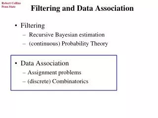
Filtering and Data Association. Filtering Recursive Bayesian estimation (continuous) Probability Theory Data Association Assignment problems (discrete) Combinatorics. Data Association Scenario. Two-frame Matching (Correspondence Problem). Match up detected blobs across video frames.

Filtering and Data Association
E N D
Presentation Transcript
Filtering and Data Association • Filtering • Recursive Bayesian estimation • (continuous) Probability Theory • Data Association • Assignment problems • (discrete) Combinatorics
Data Association Scenario Two-frame Matching (Correspondence Problem) Match up detected blobs across video frames
Data Association Scenario Frame T+1 Form a matrix ofpairwise similarity scores .23 .95 .11 .89 Frame T .25 .85 .81 .12 .90 We want to choose one match from each row and column to maximize sum of scores
Data Association Scenario Two-frame Matching (Correspondence Problem) Matching features across frames e.g. corners, Sift keys, image patches
Data Association Scenarios Multi-frame Matching
Data Association Scenarios In general, data association of blobs in video is easier than general correspondence problem associating features across two image frames. Why? Because of temporal coherence of object motion, which spatially constrains candidate matches.
Outline • Track Prediction and Gating • Global Nearest Neighbor (GNN) • Linear Assignment Problem • Probabilistic Data Association (PDAF) • Joint Probabilistic Data Assoc (JPDAF) • Multi-Hypothesis Tracking (MHT) • Network Flow for Multiframe Matching
Track Matching How do we match observations in a new frame to a set of tracked trajectories? ? track 1 track 2 observations
Track Matching First, predict next target position along each track.(e.g. based on constant velocity motion prediction) ? track 1 track 2 observations
Track Matching Form a “gating” region around each predicted target location to filter out unlikely matches that are too far away. gatingregion 2 ? track 1 ? gatingregion 1 track 2 observations Note, this decomposes the full N x N matching problem into a sparse set of smaller subproblems.
Track Matching For each candidate match (a track-to-data pairing), compute match score based on likelihood of the data given the track. d1 ? d3 d2 track 1 ? d5 d4 track 2 Match score based on Euclidean or Mahalanobis distance to predicted location (e.g. exp{-d2}). Could also incorporate similarity of appearance (e.g. intensity patch correlation or color histogram similarity)
Track Matching For each candidate match (a track-to-data pairing), compute match score based on likelihood of the data given the track. d1 d3 d2 track 1 d5 d4 ai1 ai2 track 2 3.0 2 5.0 3 6.0 8.0 3.0 Scores:
Track Matching Determine best match and extend the trajectory. (e.g. using these observations in a Kalman filter update) track 1 ai1 ai2 track 2 3.0 2 5.0 3 6.0 8.0 3.0 Scores:
both try to claim observation o4 Global Nearest Neighbor (GNN) Problem: if we do that independently for each track, we could end up with contention for the same observations when gating regions overlap. ai1 ai2 o2 3.0 2 5.0 3 6.0 1.0 9.0 8.0 3.0 o1 o3 track1 o4 o5 track2
Greedy (Best First) Strategy Assign observations to trajectories in decreasing order of goodness, making sure to not reuse an observation twice. ai1 ai2 o2 3.0 2 5.0 3 6.0 1.0 9.0 8.0 3.0 o1 o3 track1 o4 o5 SUBOPTIMAL SOLUTiON! track2
Linear Assignment Problem We have N objects in previous frame and M objects in current frame. We can build a table of match scores m(i,j) for i=1...N and j=1...M. For now, assume M=N. 1 2 3 4 5 0.95 0.76 0.62 0.41 0.06 0.23 0.46 0.79 0.94 0.35 0.61 0.02 0.92 0.92 0.81 0.49 0.82 0.74 0.41 0.01 0.89 0.44 0.18 0.89 0.14 1 2 3 4 5 problem: choose a 1-1 correspondence thatmaximizes sum of match scores.
constraints that sayX is a permutation matrix Linear Assignment Problem Mathematical Definition maximize: subject to: The permutation matrix ensures that we only match up one object from each row and from each column. note: alternately, we can minimize costs rather than maximize weights minimize:
Hungarian Algorithm hence the name
Handling Missing Matches Typically, there will be a different number of tracks than observations. Some observations may not match any track. Some tracks may not have observations. That’s OK. Most implementations of Hungarian Algorithm allow you to use a rectangular matrix, rather than a square matrix. See for example:
track1 track2 0 0 2 0 0 3 1 0 0 1 0 0 Square-matrix assignment 5x3 ignore whateverhappens in here If Square Matrix is Required... track1 track2 3.0 0 2 5.0 0 3 6.0 1.0 9.0 8.0 0 3.0 pad with array of small random numbers to get a square score matrix. 5x3
Result From Hungarian Algorithm Each track is now forced to claim a different observation. And we get the optimal assignment. ai1 ai2 o2 3.0 2 5.0 3 6.0 1.0 9.0 8.0 3.0 o1 o3 track1 o4 o5 track2
PDAF Probabilistic Data Association Filter Updating single track based on soft assignments. General idea: Instead of matching a single best observation to the track, we update based on all observations (in gating window), weighted by their match scores.
PDAF Consider all points in gating window. Also consider the additional possibility that no observations match. ai1 o2 0 1.0 1 3.0 2 5.0 3 6.0 4 9.0 o1 o3 track1 o4 pi1 = “probability” of matching observation i to track 1
PDAF The best matching “observation” is now computed as a weighted combination of the predicted locations and all candidate observations... ai1 o2 0 1.0 1 3.0 2 5.0 3 6.0 4 9.0 o1 o3 track1 o4 New location = 1/24 * predicted location + 3/24 * o1 + 5/24 * o2 + 6/24 * o3 + 9/24 * o4 Can also compute a measure of uncertainty from the spread of the candidate observations.
Problem When gating regions overlap, the same observations can contribute to updating both trajectories. ai1 ai2 o2 3.0 2 5.0 3 6.0 1.0 9.0 8.0 3.0 o1 o3 track1 o4 o5 The shared observations introduce a coupling into the decision process. track2
JPDAF Joint Probabilistic Data Association Filter If maintaining multiple tracks, doing PDAF on each one independently is nonoptimal, since observations in overlapping gate regions will be counted more than once (contribute to more than one track). JPDAF reasons over possible combinations of matches, in a principled way. e.g. Rasmussen and Hager, “Probabilistic Data Association Methods for Tracking Complex Visual Objects,” PAMI 2001. e.g. Chen, Rui and Huang, “JPDAF based HMM for Real-Time Contour Tracking,” CVPR 2001
JPDAF Example (from Blackman and Popoli).
don’t assign sameobservation twice JPDAF Candidates: track1: 0 1 2 3 track2: 0 2 3 + Oo = no match Possible assignments: (i,j) = assign i to track1, j to track2 (0, 0) (1, 0) (2, 0) (3, 0) (0, 2) (1, 2) (2, 2) (3, 2) (0, 3) (1, 3) (2, 3) (3, 3)
JPDAF Each possible (non-conflicting) assignment becomesa hypothesis with an associated probability. These likelihoods are based on appearance, prob of detection, prob of false alarm
.086 + .306 + .239 .631 JPDAF Now compute probability pij that each observation i should be assigned to track j, by adding probabilities of assignments where that is so. Example: p11 = prob that observation should be assigned to track 1.
PDAF filterfor track 1 PDAF filterfor track 2 JPDAF Combined probabilities Track1: p10 = .084 p11 = .631 p12 = .198 p13 = .087 Track2: p20 = .169 p21 = .0 p22 = .415 p23 = .416 Running PDAF filters on each track independently is now OK because any inconsistency (double counting) has been removed.
Multi-Hypothesis Tracking Basic idea: instead of collapsing the 10 hypotheses from the last example into two trajectory updates, maintain and propagate a subset of them, as each is a possible explanation for the current state of the world. This is a delayed decision approach. The hope is that future data will disambiguate difficult decisions at this time step.
Multi-Hypothesis Tracking MHT maintains a set of such hypotheses. Each is one possible set of assignments of observations to targets or false alarms.
Combinatorial Explosion Rough order of magnitude on number of hypotheses: Let’s say we have an upper bound N on number of targets and we can associate (label) each detection in each frame with a number from 1 to N. (we are ignoring false positives) N! (N-4)! N! (N-5)! N! (N-3)! * *
Mitigation Strategies Clustering: can analyze clusters (e.g. connected components) in parallel on separate processors cluster2 o7 o8 o2 o1 o9 o3 o4 o10 o5 o6 o11 o12 cluster1 cluster3
Mitigation Strategies Track Merging • merge similar trajectories (because this might allow you to merge hypotheses) • common observation history (e.g two tracks having the last N observations in common) • similar current state estimates (e.g same location and velocity in Kalman Filter)
Mitigation Strategies Pruning: Discard low probability hypotheses For example, one hypothesis that is always available is that every contact ever observed has been a false alarm! However, that is typically a very low probability event. One of the most principled approaches to this is by Cox and Hingorani (PAMI’96). They combine MHT with Murty’s k-best assignment algorithm to maintain a fixed set of k best hypotheses at each scan.
Network Flow Approach Motivation: Seeking a globally optimal solution by considering observations over all frames in “batch mode” to find the best joint set of trajectories Approach: Extend two-frame assignment formulation by using observations from all frames to form a flow graph frame1 frame2 frame3 frame4 a1 b1 d1 c1 T S a2 b2 d2 c2 a3 b3 d3 c3
Network Flow Approach Motivation: Seeking a globally optimal solution by considering observations over all frames in “batch mode” to find the best joint set of trajectories Approach: Solving for min-cost flow in the network finds the optimal paths / trajectories. frame1 frame2 frame3 frame4 a1 b1 d1 c1 T S a2 b2 d2 c2 a3 b3 d3 c3
Network Flow Approach picture from Zhang, Li and Nevatia, “Global Data Association for Multi-Object Tracking Using Network Flows,” CVPR 2008.
Network Flow Solutions • push-relabel method • Zhang, Li and Nevatia, “Global Data Association for Multi-Object Tracking Using Network Flows,” CVPR 2008. • successive shortest path algorithm • Berclaz, Fleuret, Turetken and Fua, “Multiple Object Tracking using K-shortest Paths Optimization,” IEEE PAMI, Sep 2011. • Pirsiavash, Ramanan, Fowlkes, “Globally Optimal Greedy Algorithms for Tracking a Variable Number of Objects,” CVPR 2011. • these both include approximate dynamic programming solutions