Download

1 / 63
630 likes | 767 Vues
Experiments on a New Inter-Subject Registration Method. John Ashburner 2007. Abstract.

E N D
Experiments on a New Inter-Subject Registration Method John Ashburner 2007
Abstract • The objective of this work was to devise a more precise method of inter-subject brain image registration than those currently available in the SPM software. This involved a model with many more degrees of freedom, but which still enforces a one-to-one mapping. Speed considerations were also important. The result is an approach that models each warp by single velocity field. These are converted to deformations by a scaling and squaring procedure, and the inverses can be generated in a similar way. Registration is via a Levenberg-Marquardt optimization strategy, which uses a full multi-grid algorithm to rapidly solve the necessary equations. • The method has been used for warping images of 471 subjects. This involved simultaneously matching grey matter with a grey matter template, and white matter with a white matter template. After every few iterations, the templates were re-generated from the means of the warped individual images. Evaluations involved applying pattern recognition procedures to the resulting deformations, in order to assess how well information such as the ages and sexes of the subjects could be predicted from the encoded deformations. A slight improvement in prediction accuracy was obtained when compared to a similar procedure using a small deformation model.
Overview • Motivation • Dimensionality • Inverse-consistency • Principles • Geeky stuff • Example • Validation • Future directions
Motivation • More precise inter-subject alignment • Improved fMRI data analysis • Better group analysis • More accurate localization • Improve computational anatomy • More easily interpreted VBM • Better parameterization of brain shapes • Other applications • Tissue segmentation • Structure labeling
Image Registration • Figure out how to warp one image to match another • Normally, all subjects’ scans are matched with a common template
Current SPM approach • Only about 1000 parameters. • Unable model detailed deformations
A simple 2D example Individual brain Warped Individual Reference
Residual Differences Individual brain Warped Individual
Expansion and contraction • Relative volumes encoded by Jacobian determinants of deformation
Tissue volume comparisons Warped grey matter Jacobian determinants Absolute grey matter volumes
A one-to-one mapping • Many models simply add a smooth displacement to an identity transform • One-to-one mapping not enforced • Inverses approximately obtained by subtracting the displacement • Not a real inverse Small deformation approximation
Overview • Motivation • Principles • Geeky stuff • Example • Validation • Future directions
Principles Diffeomorphic Anatomical Registration Through Exponentiated Lie Algebra Deformations parameterized by a single flow field, which is considered to be constant in time.
DARTEL • Parameterizing the deformation • φ(0)(x) = x • φ(1)(x) = ∫u(φ(t)(x))dt • u is a flow field to be estimated 1 t=0
Euler integration • The differential equation is dφ(x)/dt = u(φ(t)(x)) • By Euler integration φ(t+h) = φ(t) + hu(φ(t)) • Equivalent to φ(t+h) = (x + hu) oφ(t)
Simple integration φ(1/8) = x + u/8 φ(2/8) = φ(1/8)oφ(1/8) φ(3/8) = φ(1/8)oφ(2/8) φ(4/8) = φ(1/8)oφ(3/8) φ(5/8) = φ(1/8)oφ(4/8) φ(6/8) = φ(1/8)oφ(5/8) φ(7/8) = φ(1/8)oφ(6/8) φ(8/8) = φ(1/8)oφ(7/8) 7 compositions Scaling and squaring φ(1/8) = x + u/8 φ(2/8) = φ(1/8)oφ(1/8) φ(4/8) = φ(2/8)oφ(2/8) φ(8/8) = φ(4/8)oφ(4/8) 3 compositions Similar procedure used for the inverse. Starts with φ(-1/8) = x - u/8 For (e.g) 8 time steps
Overview • Motivation • Principles • Geeky stuff • Feel free to sleep • Example • Validation • Future directions
Registration objective function • Simultaneously minimize the sum of • Likelihood component • From the sum of squares difference • ½∑i(g(xi) – f(φ(1)(xi)))2 • φ(1) parameterized by u • Prior component • A measure of deformation roughness • ½uTHu
Regularization model • DARTEL has three different models for H • Membrane energy • Linear elasticity • Bending energy • H is very sparse An example H for 2D registration of 6x6 images (linear elasticity)
Optimisation • Uses Levenberg-Marquardt • Requires a matrix solution to a very large set of equations at each iteration u(k+1) = u(k) - (H+A)-1b • b are the first derivatives of objective function • A is a sparse matrix of second derivatives • Computed efficiently, making use of scaling and squaring
Relaxation • To solve Mx = c Split M into E and F, where • E is easy to invert • F is more difficult • Sometimes: x(k+1) = E-1(c – F x(k)) • Otherwise: x(k+1) = x(k) + (E+sI)-1(c – M x(k)) • Gauss-Siedel when done in place. • Jacobi’s method if not • Fits high frequencies quickly, but low frequencies slowly
Highest resolution Full Multi-Grid Lowest resolution
Overview • Motivation • Principles • Geeky stuff • Example • Simultaneous registration of GM & WM • Tissue probability map creation • Validation • Future directions
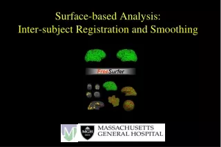
Grey matter Grey matter Grey matter Grey matter White matter White matter White matter White matter Simultaneous registration of GM to GM and WM to WM Subject 1 Subject 3 Grey matter White matter Template Subject 2 Subject 4
Template Initial Average Iteratively generated from 471 subjects Began with rigidly aligned tissue probability maps Used an inverse consistent formulation After a few iterations Final template
Initial GM images
Warped GM images
Overview • Motivation • Principles • Geeky stuff • Example • Validation • Sex classification • Age regression • Future directions
Validation • There is no “ground truth” • Looked at predictive accuracy • Can information encoded by the method make predictions? • Registration method blind to the predicted information • Could have used an overlap of fMRI results • Chose to see whether ages and sexes of subjects could be predicted from the deformations • Comparison with small deformation model
? ? ? ? Training and Classifying Control Training Data Patient Training Data
? ? ? ? Classifying Controls Patients y=f(aTx+b)
Support Vector Classifier (SVC) a is a weighted linear combination of the support vectors Support Vector Support Vector Support Vector
Some Equations • Linear classification is by y = f(aTx + b) • where a is a weighting vector, x is the test data, b is an offset, and f(.) is a thresholding operation • a is a linear combination of SVs a = Si wixi • So y = f(Si wixiTx + b)
Going Nonlinear • Nonlinear classification is by y = f(Si wi(xi,x)) • where (xi,x) is some function of xi and x. • e.g. RBF classification • (xi,x) = exp(-||xi-x||2/(2s2)) • Requires a matrix of distance measures (metrics) between each pair of images.
Cross-validation • Methods must be able to generalise to new data • Various control parameters • More complexity -> better separation of training data • Less complexity -> better generalisation • Optimal control parameters determined by cross-validation • Test with data not used for training • Use control parameters that work best for these data
Two-fold Cross-validation Use half the data for training. and the other half for testing.
Two-fold Cross-validation Then swap around the training and test data.
Leave One Out Cross-validation Use all data except one point for training. The one that was left out is used for testing.
Leave One Out Cross-validation Then leave another point out. And so on...