Divide-and-Conquer
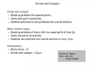
Divide-and-Conquer. Divide-and-Conquer. It’s a technique instead of an algorithm Recursive in structure Divide the problem into several smaller sub-problems that are similar to the original but smaller in size


Divide-and-Conquer
E N D
Presentation Transcript
Divide-and-Conquer Z. Guo
Divide-and-Conquer • It’s a technique instead of an algorithm • Recursive in structure • Divide the problem into several smaller sub-problems that are similar to the original but smaller in size • Conquer the sub-problems by solving them recursively. If they are small enough, just solve them in a straightforward manner. • Combine the solutions to create a solution to the original problem Z. Guo
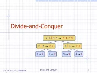
An Example: Merge Sort Sorting Problem:Sort a sequence or n elements into non-decreasing order. • Divide: Divide the n-element sequence to be sorted into two subsequences of n/2 elements each • Conquer: Sort the two subsequences recursively using merge sort. • Combine: Merge the two sorted subsequences to produce the sorted answer. Z. Guo
18 18 26 26 32 32 6 6 43 43 15 15 9 9 1 1 43 43 15 15 9 9 1 1 18 18 26 26 32 32 6 6 18 18 26 26 32 32 6 6 43 43 15 15 9 9 1 1 18 26 32 6 43 15 9 1 18 26 32 6 43 15 9 1 Merge Sort – Example Original Sequence Sorted Sequence 1 6 9 15 18 26 32 43 6 32 26 26 32 6 18 18 9 15 1 43 1 9 15 43 26 32 15 18 6 43 18 26 6 32 15 43 1 9 1 9 15 26 32 1 18 26 32 6 43 15 9 1 18 15 43 9 6 26 9 1 32 6 18 43 6 43 18 26 32 1 15 9 Z. Guo
Merge-Sort (A, p, r) INPUT: a sequence of n numbers stored in array A OUTPUT: an ordered sequence of n numbers • MergeSort (A, p, r) // sort A[p..r] by divide & conquer • ifp < r • thenq (p+r)/2 • MergeSort (A, p, q) • MergeSort (A, q+1, r) • Merge (A, p, q, r) // merges A[p..q] with A[q+1..r] Initial Call: MergeSort(A, 1, n) Z. Guo
Sentinels, to avoid having to check if either subarray is fully copied at each step. Procedure Merge Input: Array containing sorted subarrays A[p..q] and A[q+1..r]. Output: Merged sorted subarray in A[p..r]. Merge(A, p, q, r) 1 n1 q – p + 1 2 n2 r –q • fori 1 ton1 • doL[i] A[p + i – 1] • forj 1 ton2 • doR[j] A[q + j] • L[n1+1] • R[n2+1] • i 1 • j 1 • fork p tor • doifL[i] R[j] • thenA[k] L[i] • i i + 1 • elseA[k] R[j] • j j + 1 Z. Guo
Merge – Example A … 6 8 26 32 1 9 42 43 … 1 6 8 9 26 32 42 43 k k k k k k k k k L R 6 8 26 32 6 8 26 32 1 9 42 43 1 9 42 43 i i i i i j j j j j Z. Guo
Correctness of Merge Loop Invariant for the for loop At the start of each iteration of the for loop: Subarray A[p..k – 1] contains the k –p smallest elements of L and R in sorted order. L[i] and R[j] are the smallest elements of L and R that have not been copied back into A. Merge(A, p, q, r) 1 n1 q – p + 1 2 n2 r –q • fori 1 ton1 • doL[i] A[p + i – 1] • forj 1 ton2 • doR[j] A[q + j] • L[n1+1] • R[n2+1] • i 1 • j 1 • fork p tor • doifL[i] R[j] • thenA[k] L[i] • i i + 1 • elseA[k] R[j] • j j + 1 • Initialization: • Before the first iteration: • A[p..k – 1] is empty. • i = j = 1. • L[1] and R[1] are the smallest • elements of L and R not copied to A. Z. Guo
Correctness of Merge • Maintenance: • Case 1:L[i] R[j] • By LI, A contains p – k smallest elements of L and R in sorted order. • By LI, L[i] and R[j] are the smallest elements of L and R not yet copied into A. • Line 13 results in A containing p – k + 1 smallest elements (again in sorted order). • Incrementing i and k reestablishes the LI for the next iteration. • Similarly for L[i] > R[j]. Merge(A, p, q, r) 1 n1 q – p + 1 2 n2 r –q • fori 1 ton1 • doL[i] A[p + i – 1] • forj 1 ton2 • doR[j] A[q + j] • L[n1+1] • R[n2+1] • i 1 • j 1 • fork p tor • doifL[i] R[j] • thenA[k] L[i] • i i + 1 • elseA[k] R[j] • j j + 1 • Termination: • On termination, k = r + 1. • By LI, A contains r – p + 1 smallest • elements of L and R in sorted order. • L and R together contain r – p + 3 elements. • All but the two sentinels have been copied • back into A. Z. Guo
Analysis of Merge Sort • Running time T(n) of Merge Sort: • Divide: computing the middle takes (1) • Conquer: solving 2 subproblems takes 2T(n/2) • Combine: merging n elements takes (n) • Total: T(n) = (1)if n = 1 T(n) = 2T(n/2) + (n)if n > 1 T(n) = (n lg n) (CLRS, Chapter 4) • MergeSort (A, p, r) // sort A[p..r] by divide & conquer • ifp < r • thenq (p+r)/2 • MergeSort (A, p, q) • MergeSort (A, q+1, r) • Merge (A, p, q, r) // merges A[p..q] with A[q+1..r] Z. Guo
Recurrence Relations • Recurrences (Chapter 4) • Substitution Method • Iteration Method • Master Method • Arising from Divide and Conquer (e.g. MERGE-SORT) T(n) = (1) if n c T(n) = a T(n/b) + D(n) + C(n) otherwise Z. Guo
Substitution Method • Guessing the form of the solutions, then using mathematical induction to find the constants and show the solution works. • It works well when it is easy to guess. But, there is no general way to guess the correct solution. Z. Guo
An Example • Solve: T(n) = 3T(n/3) + n T(n) = = c n lg n GUESS Z. Guo
An Example • Solve: T(n) = 3T(n/3) + n T(n) 3c n/3 lg n/3 + n c n lg (n/3) + n = c n lg n - c n lg3 + n = c n lg n - n (c lg 3 - 1) c n lg n * The last step istrue for c 1 / lg3. Z. Guo
Making a Good Guess • Guessing a similar solution to the one that you have seen before • T(n) = 3T(n/3 + 5) + n similar to T(n) = 3T(n/3) + n when n is large, the difference between n/3 and (n/3 + 5) is insignificant • Another way is to prove loose upper and lower bounds on recurrence and then reduce the range of uncertainty. • Start with T(n) = (n) & T(n) = O(n2) T(n) = (n log n) Z. Guo
Changing Variables • Use algebraic manipulation to turn an unknown recurrence similar to what you have seen before. • Consider T(n) = 2T(n1/2) + lg n Z. Guo
Changing Variables • Use algebraic manipulation to turn an unknown recurrence similar to what you have seen before. • Consider T(n) = 2T(n1/2) + lg n • Rename m = lg n and we have T(2m) = 2T(2m/2) + m • Set S(m) = T(2m) and we have S(m) = 2S(m/2) + m S(m) = O(m lg m) • Changing back from S(m) to T(n), we have T(n) = T(2m) = S(m) = O(m lg m) = O(lg n lg lg n) Z. Guo
Avoiding Pitfalls • Be careful not to misuse asymptotic notation. For example: • We can falsely prove T(n) = O(n) by guessing T(n) c n for T(n) = 2T(n/2) + n T(n) 2c n/2 + n c n + n = O(n) Wrong! • The err is that we haven’t proved T(n) c n Z. Guo
Exercises • Solution of T(n) = T(n/2) + 1 isO(lg n) • Solution of T(n) = 2T(n/2+ 17) + n isO(n lg n) • Solve T(n) = 2T(n1/2) + 1 by making a change of variables. Don’t worry whether values are integral. Z. Guo
Recursion-tree Method • Making a good guess is sometimes difficult ... • Use recursion trees to devise good guesses. • Recursion Trees • Show successive expansions of recurrences using trees. • Keep track of the time spent on the subproblems of a divide and conquer algorithm. • Help organize the algebraic bookkeeping necessary to solve a recurrence. Comp 550
Recursion Tree – Example • Running time of Merge Sort: T(n) = (1)if n = 1 T(n) = 2T(n/2) + (n)if n > 1 • Rewrite the recurrence as T(n) = cif n = 1 T(n) = 2T(n/2) + cnif n > 1 c > 0:Running time for the base case and time per array element for the divide and combine steps. Comp 550
cn Cost of divide and merge. cn cn/2 cn/2 T(n/2) T(n/2) T(n/4) T(n/4) T(n/4) T(n/4) Cost of sorting subproblems. Recursion Tree for Merge Sort For the original problem, we have a cost of cn, plus two subproblems each of size (n/2) and running time T(n/2). Each of the size n/2 problems has a cost of cn/2 plus two subproblems, each costing T(n/4). T(n) = 2T(n/2) + cn Comp 550
cn cn/2 cn/2 cn/4 cn/4 cn/4 cn/4 c c c c c c Recursion Tree for Merge Sort Continue expanding until the problem size reduces to 1. cn cn lg n cn cn Total : cnlgn+cn Comp 550
cn cn/2 cn/2 cn/4 cn/4 cn/4 cn/4 c c c c c c Recursion Tree for Merge Sort Continue expanding until the problem size reduces to 1. • Each level has total cost cn. • Each time we go down one level, the number of subproblems doubles, but the cost per subproblem halves cost per level remains the same. • There are lg n + 1 levels, height is lg n. (Assuming n is a power of 2.) • Can be proved by induction. • Total cost = sum of costs at each level = (lg n + 1)cn = cnlgn + cn = (n lgn). Comp 550
Recursion Trees and Recurrences • Useful even when a specific algorithm is not specified • For T(n) = 2T(n/2) + n2, we have Z. Guo
Recursion Trees T(n) = (n2) Z. Guo
Recursion Trees – Caution Note • Recursion trees only generate guesses. • Verify guesses using substitution method. • If careful when drawing out a recursion tree and summing the costs, can be used as direct proof. Comp 550
Recursion Trees • Exercise T(n) = T(n/2) + T(n/4) + n2 Z. Guo
The Master Method • Based on the Master theorem. • “Cookbook” approach for solving recurrences of the form T(n) = aT(n/b) + f(n) • a 1, b > 1 are constants. • f(n) is asymptotically positive. • T(n) is defined for nonnegative integers • n/b may not be an integer, but we ignore floors and ceilings. Why? Comp 550
The Master Theorem • Theorem 4.1 • Let a 1 and b > 1be constants, let f(n) be a function, and Let T(n) be defined on nonnegative integers by the recurrence T(n) = aT(n/b) + f(n), where we can replace n/b by n/b or n/b. T(n) can be bounded asymptotically in three cases: • If f(n) = O(nlogba–) for some constant > 0, then T(n) = (nlogba). • If f(n) = (nlogba), then T(n) = (nlogbalg n). • If f(n) = (nlogba+) for some constant > 0, and if, for some constant c < 1 and all sufficiently large n, we have a·f(n/b) c f(n), then T(n) = (f(n)). We’ll return to recurrences as we need them… If none of these three cases apply, you’re on your own. Comp 550
Master Theorem Let a 1 and b >1 be constants andlet T(n) be the recurrence T(n) = a T(n/b) + c nk defined for n 0. 1. If a>bk, then T(n) = ( nlogba ). 2. Ifa=bk, then T(n) = ( nk lg n ). 3. If a< bk, then T(n) = ( nk ). Z. Guo
Examples • T(n) = 16T(n/4) + n • a = 16, b = 4, thus nlogba = nlog416= (n2) • f(n) = n = O(nlog416-)where = 1 case 1. • Therefore, T(n) = (nlogba)=(n2) • T(n) = T(3n/7) + 1 • a = 1, b=7/3, and nlogba = nlog7/31 = n0 = 1 • f(n) = 1 = (nlogba)case 2. • Therefore, T(n) = (nlogba lg n) = (lg n) Z. Guo
Examples (Cont.) • T(n) = 3T(n/4) + n lg n • a = 3, b=4, thus nlogba = nlog43 = O(n0.793) • f(n) = n lg n = (nlog43 + )where 0.2case 3. • Therefore, T(n) = (f(n)) = (n lg n) • T(n) = 2T(n/2) + n lg n • a = 2, b=2, f(n) = n lg n, and nlogba = nlog22 = n • f(n)is asymptotically larger thannlogba, but not polynomially larger. The ratio lg n is asymptotically less than n for any positive . Thus, the Master Theorem doesn’tapply here. Z. Guo
Exercises • Use the Master Method to solve the following: • T(n) = 4T(n/2) + n • T(n) = 4T(n/2) + n2 • T(n) = 4T(n/2) + n3 • Try this if you finished the ones above:T(n) = 4T(n/2) + n2/lgn Z. Guo