Dynamic Light Scattering

1. Dynamic Light Scattering ZetaPALS w/ 90Plus particle size analyzer Also equipped w/ BI-FOQELS & Otsuka DLS-700 (Rm CCR230)

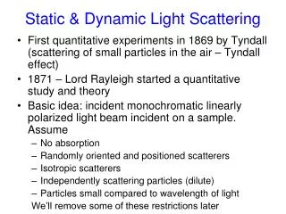
2. Dynamic Light Scattering (DLS) Photon Correlation Spectroscopy (PCS) Quasi-Elastic Light Scattering (QELS) • Measure Brownian motion by … • Collect scattered light from suspended particles to … • Obtain diffusion rate to … • Calculate particle size

3. Brownian motion • Velocity of the Brownian motion is defined by the Translational Diffusion Coefficient (D) • Brownian motion is indirectly proportional to size • Larger particles diffuse slower than smaller particles • Temperature and viscosity must be known • Temperature stability is necessary • Convection currents induce particle movement that interferes with size determination • Temperature is proportional to diffusion rate • Increasing temperature increases Brownian motion

4. Brownian motion Random movement of particles due to bombardment of solvent molecules

5. Stokes-Einstein Equation dH = hydrodynamic diameter (m) k = Boltzmann constant (J/K=kg·m2/s2·K) T = temperature (K) η = solvent viscosity (kg/m·s) D = diffusion coefficient (m2/s)

6. Hydrodynamic diameter Particle diameter • The diameter measured by DLS correlates to the effective particle movement within a liquid • Particle diameter + electrical double layer • Affected by surface bound species which slows diffusion Hydrodynamic diameter

7. Nonspherical particles = Rapid Equivalent sphere Slow Hydrodynamic diameter is calculated based on the equivalent sphere with the same diffusion coefficient

8. Experimental DLS • Measure the Brownian motion of particles and calculate size • DLS measures the intensity fluctuations of scattered light arising from Brownian motion • How do these fluctuations in scattered light intensity arise?

9. What causes light scattering from (small) particles? • Explained by JW Strutt (Lord Rayleigh) • Electromagnetic wave (light) induces oscillations of electrons in a particle • This interaction causes a deviation in the light path through an angle calculated using vector analysis • Scattering coefficient varies inversely with the fourth power of the wavelength

10. Interaction of light with matterRayleigh approximation • For small particles (d ≤ λ/10), scattering is isotropic • Rayleigh approximation tells us that I α d6 I α 1/λ4 where I = intensity of scattered light d = particle diameter λ = laser wavelength

11. Mie scattering from large particles • Used for particles where d ~ λ0 • Complete analytical solution of Maxwell’s equations for scattering of electromagnetic radiation from spherical particles • Assumes homogeneous, isotropic and optically linear material Stratton, A. Electromagnetic theory, McGraw-Hill, New York (1941) www.lightscattering.de/MieCalc

12. Brownian motion and scattering Constructive interference Destructive interference

13. Brownian motion and scattering Multiple particles

14. Instrument layout

15. Intensity fluctuations • Apply the autocorrelation function to determine diffusion coefficient • Large particles – smooth curve • Small particles – noisy curve

16. Determining particle size • Determine autocorrelation function • Fit measured function to G(τ) to calculate Γ • Calculate D, given n*, θ, and Γ • Calculate dH, given T* and η* *User defined values.

17. How a correlator works • Random motion of small particles in a liquid gives rise to fluctuations in the time intensity of the scattered light • Fluctuating signal is processed by forming the autocorrelation function • Calculates diffusion

18. How a correlator works • Large particles – the signal will be changing slowly and the correlation will persist for a long time • Small, rapidly moving particles – the correlation will disappear quickly

19. The correlation function • For monodisperse particles the correlation function is • Where • A= baseline of the correlation function • B=intercept of the correlation function • Γ=Dq2 • D=translational diffusion coefficient • q=(4πn/λ0)sin(θ/2) • n=refractive index of solution • λ0=wavelength of laser • θ=scattering angle

20. The correlation function • For polydisperse particles the correlation function becomes where g1(τ) is the sum of all exponential decays contained in the correlation function

21. Broad particle size distribution • Correlation function becomes nontrivial • Measurement noise, baseline drifts, and dust make the function difficult to solve accurately • Cumulants analysis • Convert exponential to Taylor series • First two cumulants are used to describe data • Γ = Dq2 • μ2 = (D2*-D*2)q4 • Polydispersity = μ2/ Γ2

22. Cumulants analysis • The decay in the correlation function is exponential • Simplest way to obtain size is to use cumulants analysis1 • A 3rd order fit to a semi-log plot of the correlation function • If the distribution is polydisperse, the semi-log plot will be curved • Fit error of less than 0.005 is good. 1ISO 13321:1996 Particle size analysis -- Photon correlation spectroscopy

23. Cumulants analysis • Third order fit to correlation function • b = z-average diffusion coefficient • 2c/b2 = polydispersity index • This method only calculates a mean and width • Intensity mean size • Only good for narrow, monomodal samples • Use NNLS for multimodal samples

24. Cumulants analysis

25. Polydispersity index • 0 to 0.05 – only normally encountered w/ latex standards or particles made to be monodisperse • 0.05 to 0.08 – nearly monodisperse sample • 0.08 to 0.7 – This is a mid-range polydispersity • >0.7 – Very polydisperse. Care should be taken in interpreting results as the sample may not be suitable for the technique (e.g., a sedimenting high size tail may be present)

26. Non-Negatively constrained Least Squares (NNLS) algorithm • Used for Multimodal size distribution (MSD) • Only positive contributions to the intensity-weighted distribution are allowed • Ratio between any two successive diameters is constant • Least squares criterion for judging each criterion is used • Iteration terminates on its own

27. Correlation functionCorrelograms Correlograms show the correlation data providing information about the sample The shape of the curve provides clues related to sample quality • Decay is a function of the particle diffusion coefficient (D) • Stokes-Einstein relates D to dH • z-average diameter is obtained from an exponential fit • Distributions are obtained from multi-exponential fitting algorithms Noisy data can result from • Low count rate • Sample instability • Vibration or interference from external source

28. Correlation functionCorrelograms

29. Data interpretationCorrelograms • Very small particles • Medium range polydispersity • No large particles/aggregrates present (flat baseline)

30. Data interpretationCorrelograms • Large particles • Medium range polydispersity • Presence of large particles/agglomerates (noisy baseline)

31. Data interpretationCorrelograms • Very large particles • High polydispersity • Presence of large particles/agglomerates (noisy baseline)

32. Upper size limit of DLS • DLS will have an upper limit wrt size and density • When particle motion is not random (sedimentation or creaming), DLS is not the correct technique to use • Upper limit is set by the onset of sedimentation • Upper size limit is therefore sample dependent • No advantage in suspending particles in a more viscous medium to prevent sedimentation because Brownian motion will be slowed down to the same extent making measurement time longer

33. Upper size limit of DLS • Need to consider the number of particles in the detection volume • Amount of scattered light from large particles is sufficient to make successful measurements, but … • Number of particles in scattering volume may be too low • Number fluctuations – severe fluctuations of the number of particles in a time step can lead to problems defining the baseline of the correlation function • Increase particle concentration, but not too high or multiple scattering events might arise

34. Detection volume Detector Laser

35. Lower particle size limit of DLS • Lower size limit depends on • Sample concentration • Refractive index of sample compared to diluent • Laser power and wavelength • Detector sensitivity • Optical configuration of instrument Lower limit is typically ~ 2 nm

36. Sample preparation • Measurements can be made on any sample in which the particles are mobile • Each sample material has an optimal concentration for DLS analysis • Low concentration → not enough scattering • High concentration → multiple scattering events affect particle size

37. Sample preparation • Upper limit governed by onset of particle/particle interactions • Affects diffusion speed • Affects apparent size • Multiple scattering events and particle/particle interactions must be considered • Determining the correct particle concentration may require several measurements at different concentrations

38. Sample preparation An important factor determining the maximum concentration for accurate measurements is the particle size

39. Sample concentrationSmall particles • For particle sizes <10 nm, one must determine the minimum concentration to generate enough scattered light • Particles should generate ~ 10 kcps (count rate) in excess of the scattering from the solvent • Maximum concentration determined by the physical properties of the particles • Avoid particle/particle interactions • Should be at least 1000 particles in the scattering volume

40. Sample preparation • When possible, perform DLS on as prepared sample • Dilute aqueous or organic suspensions • Alcohol and aggressive solvents require a glass/quartz cell • 0.0001 to 1%(v/v) • Dilution media (1) should be the same (or as close as possible) as the synthesis media, (2) HPLC grade and (3) filtered before use • Chemical equilibrium will be established if diluent is taken from the original sample • Suspension should be sonicated prior to analysis

41. Checking instrument operation • DLS instruments are not calibrated • Measurement based on first principles • Verification of accuracy can be checked using standards • Duke Scientific (based on TEM) • Polysciences

42. Count rate and z-average diameter Repeatability • Perform at least 3 repeat measurements on the same sample • Count rates should fall within a few percent of one another • z-average diameter should also be with 1-2% of one another

43. Count rateRepeatability problems • Count rate DECREASES with successive measurements • Particle sedimentation • Particle creaming • Particle dissolution or breaking up • Resolution • Prepare a better, stabilized dispersion • Get rid of large particles • Coulter

44. Count rateRepeatability problems • Count rate is RANDOM with successive measurements • Dispersion instability • Sample contains large particles • Bubbles • Resolution • Prepare a better, stabilized dispersion • Remove large particles • De-gas sample

45. Z-average diameterRepeatability problems • Size DECREASES with successive measurements • Temperature not stable • Sample unstable • Resolution • Allow plenty of time for temperature equilibration • Prepare a better, stabilized dispersion

46. Repeatability of size distributions • The sized distributions are derived from a NNLS analysis and should be checked for repeatability as well • If distributions are not repeatable, repeat measurements with longer measurement duration

47. References • http://www.bic.com/90Plus.html • http://www.brainshark.com/brainshark/vu/view.asp?text=M913802&pi=62212 • http://www.malvern.co.uk/malvern/ondemand.nsf/frmondemandview • http://www.brainshark.com/brainshark/vu/view.asp?text=M913802&pi=96389 • http://www.brainshark.com/brainshark/vu/view.asp?text=M913802&pi=73504 • http://physics.ucsd.edu/neurophysics/courses/physics_173_273/dynamic_light_scattering_03.pdf • http://www.brookhaven.co.uk/dynamic-light-scattering.html • Dynamic Light Scattering: With Applications to Chemistry, Biology, and Physics, Bruce J. Berne and Robert Pecora, DOVER PUBLICATIONS, INC. Mineola. New York • Scattering of Light & Other Electromagnetic Radiation, Milton Kerker, Academic Press (1969)

49. Evaluating the correlation function • If the intensity distribution is a fairly smooth peak, there is little point in conversion to a volume distribution using Mie theory • However, if the intensity plot shows a substantial tail or more than one peak, then a volume distribution will give a more realistic view of the importance of the tail or second peak • Number distributions are of little use because small error in data acquisition can lead to huge error in the distribution by number and are not displayed

50. Correlogram from a sample of small particles