SlideServe
Menu
Préférences
© SlideServe · v2026

Static & Dynamic Light Scattering

sibley avatar
23 diapositives · 1.4K Views · Aug 30, 2014

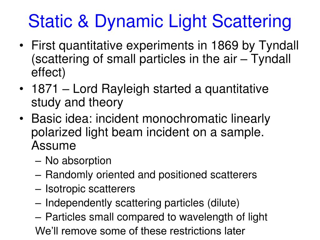
Static & Dynamic Light Scattering. First quantitative experiments in 1869 by Tyndall (scattering of small particles in the air – Tyndall effect) 1871 – Lord Rayleigh started a quantitative study and theory
Static & Dynamic Light Scattering - slide 1
01 / 23Static & Dynamic Light Scattering
1 / 17

Télécharger la présentation

Static & Dynamic Light Scattering
Une image / un lien ci-dessous est fourni (tel quel) pour télécharger la présentation

Politique de téléchargement : le contenu du site vous est fourni TEL QUEL pour votre information et votre usage personnel ; il ne peut être vendu, concédé sous licence ni partagé sur d’autres sites sans l’accord de son auteur.Le contenu vous est fourni TEL QUEL, pour votre information et votre usage personnel uniquement. Téléchargez la présentation en cliquant sur ce lien. Lors du téléchargement, si vous ne parvenez pas à télécharger une présentation, l’éditeur a peut-être supprimé le fichier de son serveur.Pendant le téléchargement, si vous ne parvenez pas à obtenir une présentation, le fichier a peut-être été supprimé par l’éditeur.

F I N

Plus de contenu associé

Transcription de la présentation
  1. Static & Dynamic Light Scattering • First quantitative experiments in 1869 by Tyndall (scattering of small particles in the air – Tyndall effect) • 1871 – Lord Rayleigh started a quantitative study and theory • Basic idea: incident monochromatic linearly polarized light beam incident on a sample. Assume • No absorption • Randomly oriented and positioned scatterers • Isotropic scatterers • Independently scattering particles (dilute) • Particles small compared to wavelength of light We’ll remove some of these restrictions later

  2. dipole Obs. Pt. r f Classical Wave description • The incident electric field is E = Eocos(2px/l – 2pt/T) • Interaction with molecules drives their electrons at the same f to induce an oscillating dipole pinduced = a Eocos(2px/l – 2pt/T) - a = polarizability • This dipole will radiate producing a scattered E field from the single molecule

  3. Static (or time-average)Rayleigh scattering • E ~ 1/r so I ~ 1/r2 - necessary since I ~energy/time/area and A ~ r2 • E ~ 1/l2 dependence so I ~ 1/l4 – blue skies and red sunsets (sunrises) • Elastic scattering – same f • sin f dependence – when f = 0 or p – at poles of dipole – no scattering – max in horizontal plane • a related to n , but how?

  4. Polarizability and index of refraction • Note that if n ~ 1 where c is the weight concentration • Then where N = number concentration • So, • For a particle in a solvent with nsolv, we have n2 – n2solv = 4pNa so

  5. Scattered Intensity • Detect intensity, not E, where • Substituting for a, we have

  6. Scattered Intensity II • If there are N scatterers/unit volume and all are independent with N = NAc/M, then • We define the Rayleigh ratio Rq:

  7. q Basic Measurement • If the intensity ratio Iq/Io, nsolv, dn/dc, l, c, f, and r are all known, you can find M. • Usually write Kc/Rq = 1/M • Measurements are usually made as a function of concentration c and scattering angle q • The concentration dependence is given by where B is called the thermodynamic virial – same as we saw before for c dependence of D (but called A)

  8. Angle Dependence • If the scatterers are small (d < l/20), they are called Rayleigh scatterers and the above is correct – the scattering intensity is independent of scattering angle • If not, then there is interference from the light scattered from different parts of the single scatterer • Different shapes give different particle scattering factors P(q) qR~q From P(q), we can get a Radius of Gyration for the scatterer

  9. Analysis of LS Data • Measure I(q, c) and plot Kc/Rq vs sin2(q/2) + (const)c • Extrapolations: c 0 q 0

  10. Final result Slope~RG Slope~B intercept Problems: Dust, Standard to measure Io, low angle measurement flare

  11. Polydispersity • If the solution is polydisperse – has a mixture of different scatterers with different M’s - then we measure an average M – but which average? • So the weight-averaged M is measured! Possible averages: Number-average Weight-average Z-average

  12. Dynamic Light Scattering - Basic ideas – what is it? - The experiment – how do you do it? - Some examples systems – why do it?

  13. Coherent beam Extra path length screen + + = = Double Slit Experiment

  14. Scatterers in solution (Brownian motion) Scattered light Laser at fo Narrow line incident laser Doppler broadened scattered light Df f fo 0 is way off scale Df ~ 1 part in 1010 - 1015 Light Scattering Experiment

  15. Detected intensity Iaverage time More Detailed Picture detector q Inter-particle interference How can we analyze the fluctuations in intensity? Data = g(t) = <I(t) I(t + t)>t = intensity autocorrelation function

  16. t For small t t For larger t g(t) t tc Intensity autocorrelation • g(t) = <I(t) I(t + t)>t

  17. What determines correlation time? • Scatterers are diffusing – undergoing Brownian motion – with a mean square displacement given by <r2> = 6Dtc (Einstein) • The correlation time tc is a measure of the time needed to diffuse a characteristic distance in solution – this distance is defined by the wavelength of light, the scattering angle and the optical properties of the solvent – ranges from 40 to 400 nm in typical systems • Values of tc can range from 0.1 ms (small proteins) to days (glasses, gels)

  18. Diffusion • What can we learn from the correlation time? • Knowing the characteristic distance and correlation time, we can find the diffusion coefficient D • According to the Stokes-Einstein equation where R is the radius of the equivalent hydrodynamic sphere and h is the viscosity of the solvent • So, if h is known we can find R(or if R is known we can find h)

  19. Why Laser Light Scattering? • Probes all motion • Non-perturbing • Fast • Study complex systems • Little sample needed Problems: Dust and best with monodisperse samples

  20. Aggregating/Gelling SystemsStudied at Union College • Proteins: • Actin – monomers to polymers and networks Study monomer size/shape, polymerization kinetics, gel/network structures formed, interactions with other actin-binding proteins Why? Epithelial cell under fluorescent microscope Actin = red, microtubules = green, nucleus = blue

  21. Aggregating systems, con’t what factors cause or promote aggregation? how can proteins be protected from aggregating? what are the kinetics? • BSA (bovine serum albumin) • beta-amyloid +/- chaperones • insulin • Polysaccharides: • Agarose • Carageenan Focus on the onset of gelation – what are the mechanisms causing gelation?how can we control them?what leads to the irreversibility of gelation?

  22. Current Projects • b-amyloid – small peptide that aggregates in the brain – believed to cause Alzheimer’s disease-

  23. Current Projects 2. Insulin aggregation • EFFECTS OF ARGININE ON THE KINETICS OF BOVINE INSULIN AGGREGATION STUDIED BY DYNAMIC LIGHT SCATTERING • By • Michael M. Varughese • ********* • Submitted in partial fulfillment • of the requirements for • Honors in the Department of Biological Sciences • and done in conjunction with the Department of Physics and Astronomy • UNION COLLEGE • June, 2011