Spanning Trees, greedy algorithms
1. HEY, SIGN UP FOR LUNCH. LOTS OF OPENINGS. Spanning Trees, greedy algorithms. Lecture 21 CS2110 – Spring 2019. About A6, Prelim 2. Prelim 2: Thursday, 23 April.


Spanning Trees, greedy algorithms
E N D
Presentation Transcript
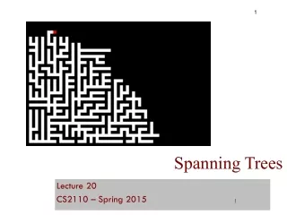
1 HEY, SIGN UP FOR LUNCH. LOTS OF OPENINGS Spanning Trees, greedy algorithms Lecture 21 CS2110 – Spring 2019
About A6, Prelim 2 Prelim 2: Thursday, 23 April. Visit exams page of course website and read carefully to find out when you take it (5:30 or 7:30) and what to do if you have a conflict. Time assignments the opposite of Prelim 1! Time assignments the opposite of Prelim 1! Time assignments the opposite of Prelim 1! Time assignments the opposite of Prelim 1! HEY, SIGN UP FOR LUNCH. LOTS OF OPENINGS
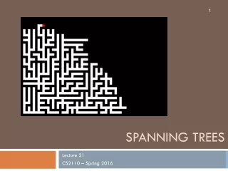
JavaHyperText material Look at entries spanning This one gives you a .zip file that contains a Java app to create random mazes. greedy We go over two algorithms for generating a spanning tree of a graph. You have to know them only at a high level of abstraction.
Amortized time Visit JavaHyperText, put “amort” into Filter Field, read the first ---one-page--- pdf file. In A5 –Heap.java, insert takes amortized time O(1). WHAT DOES THAT MEAN?
Undirected trees An undirected graph is a tree if there is exactly one simple path between any pair of vertices What’s the root? It doesn’t matter!Any vertex can be root.
Facts about trees Tree with #V = 1, #E = 0 • #E = #V – 1 • connected • no cycles Tree with #V = 3, #E = 2 Any two of these properties imply the third and thus imply that the graph is a tree
Facts about trees • #E = #V – 1 • connected • no cycles Any two of these properties imply the third and thus imply that the graph is a tree
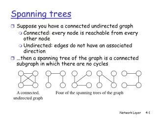
Spanning trees A spanning treeof a connected undirected graph (V, E) is a subgraph (V, E') that is a tree • Same set of vertices V • E' ⊆ E • (V, E') is a tree • Same set of vertices V • Maximal set of edges that contains no cycle • Same set of vertices V • Minimal set of edges that connect all vertices Three equivalent definitions
Spanning trees: examples http://mathworld.wolfram.com/SpanningTree.html
Finding a spanning tree: Subtractive method • Start with the whole graph – it isconnected Maximal set of edges that contains no cycle • While there is a cycle: Pick an edge of a cycle and throw it out – the graph is still connected (why?) One step of the algorithm nondeterministicalgorithm
Aside: Test whether an undirected graph has a cycle /** Visit all nodes reachable along unvisited paths from u. * Pre: u is unvisited. */ public static voiddfs(int u) { Stack s= (u); // inv: All nodes to be visited are reachable along an // unvisited path from a node in s. while (s is not empty) { u= s.pop(); if (u has not been visited) { visit u; for each edge (u, v) leaving u: s.push(v); } } } We modify iterative dfs to calculate whether the graph has a cycle
Aside: Test whether an undirected graph has a cycle /** Return true if the nodes reachable from u have a cycle. */ public static booleanhasCycle(int u) { Stack s= (u); // inv: All nodes to be visited are reachable along an // unvisited path from a node in s. while (s is not empty) { u= s.pop(); if (u has been visited) visit u; for each edge (u, v) leaving u { s.push(v); } } } returntrue; returnfalse;
Finding a spanning tree: Subtractive method • Start with the whole graph – it isconnected Maximal set of edges that contains no cycle • While there is a cycle: Pick an edge of a cycle and throw it out – the graph is still connected (why?) One step of the algorithm How many edges have to be discarded? Starts with e edges Get down to n-1 edge. Throw out e – (n-1) edges. Dense graph? Throw out O(n*n) edges! In general, too many to throw out! Don’t use!
Finding a spanning tree: Additive method • Start with no edges Minimal set of edges that connect all vertices • While the graph is not connected: Choose an edge that connects 2 connected components and add it – the graph still has no cycle (why?) nondeterministic algorithm Tree edges will be red. Dashed lines show original edges. Left tree consists of 5 connected components, each a node Add n-1 edges
Minimum spanning trees • Suppose edges are weighted (> 0) • We want a spanning tree of minimum cost (sum of edge weights) • Some graphs have exactly one minimum spanning tree. Others have several trees with the same minimum cost, each of which is a minimum spanning tree • Useful in network routing & other applications. For example, to stream a video
Greedy algorithm A greedy algorithm follows the heuristic of making a locally optimal choice at each stage, with the hope of finding a global optimum. Example. Make change using the fewest number of coins. Make change for n cents, n < 100 (i.e. < $1) Greedy: At each step, choose the largest possible coin If n >= 50 choose a half dollar and reduce n by 50; If n >= 25 choose a quarter and reduce n by 25; As long as n >= 10, choose a dime and reduce n by 10; If n >= 5, choose a nickel and reduce n by 5; Choose n pennies.
Greediness works here You’re standing at point x. Your goal is to climb the highest mountain. Two possible steps: down the hill or up the hill. The greedy step is to walk up hill. That is a local optimum choice, not a global one. Greediness works in this case. x
Greediness doesn’t work here You’re standing at point x, and your goal is to climb the highest mountain. Two possible steps: down the hill or up the hill. The greedy step is to walk up hill. But that is a local optimum choice, not a global one. Greediness fails in this case. x
Greedy algorithm —doesn’t always work! A greedy algorithm follows the heuristic of making a locally optimal choice at each stage, with the hope of finding a global optimum. Doesn’t always work Example. Make change using the fewest number of coins. Coins have these values: 7, 5, 1 Greedy: At each step, choose the largest possible coin Consider making change for 10. The greedy choice would choose: 7, 1, 1, 1. But 5, 5 is only 2 coins.
Finding a minimal spanning tree Suppose edges have > 0 weights Minimal spanning tree: sum of weights is a minimum We show two greedy algorithms for finding a minimal spanning tree. They are abstract, at a high level. They are versions of the basic additive method we have already seen: at each step add an edge that does not create a cycle. Kruskal: add an edge with minimum weight. Can have a forest of trees. Prim (JPD): add an edge with minimum weight but so that the added edges (and the nodes at their ends) form one tree
MST using Kruskal’s algorithm Minimal set of edges that connect all vertices At each step, add an edge (that does not form a cycle) with minimum weight edge with weight 2 edge with weight 3 5 5 5 5 5 3 3 3 3 3 4 4 4 4 4 4 4 4 4 4 6 6 6 6 6 2 2 2 2 2 One of the 4’s The 5 Red edges need not form tree (until end)
Kruskal Minimal set of edges that connect all vertices Start with the all the nodes and no edges, sothere is a forest of trees, each of which is asingle node (a leaf). At each step, add an edge (that does not form a cycle) with minimum weight We do not look more closely at how best to implement Kruskal’s algorithm —which data structures can be used to get a really efficient algorithm. Leave that for later courses, or you can look them up online yourself. We now investigate Prim’s algorithm
MST using “Prim’s algorithm”(should be called “JPD algorithm”) Developed in 1930 by Czech mathematician VojtěchJarník.PráceMoravskéPřírodovědeckéSpolečnosti, 6, 1930, pp. 57–63. (in Czech) Developed in 1957 by computer scientist Robert C. Prim.Bell System Technical Journal, 36 (1957), pp. 1389–1401 Developed about 1956 by Edsger Dijkstra and published in in 1959. NumerischeMathematik1, 269–271 (1959) 🙏
Prim’s algorithm Kruskal Minimal set of edges that connect all vertices At each step, add an edge (that does not form a cycle) with minimum weight, but keep added edge connected to the start (red) node edge with weight 3 edge with weight 5 5 5 5 5 5 3 3 3 3 3 4 4 4 4 4 4 4 4 4 4 6 6 6 6 6 2 2 2 2 2 One of the 4’s The 2
Difference between Prim and Kruskal Minimal set of edges that connect all vertices Prim requires that the constructed red treealways be connected. Kruskal doesn’t But: Both algorithms find a minimal spanning tree 3 5 Here, Prim chooses (0, 2) Kruskal chooses (3, 4) Here, Prim chooses (0, 1) Kruskal chooses (3, 4) 4 6 4 0 0 2 2 5 1 1 2 2 4 6 4 3 3 4 4 3
Difference between Prim and Kruskal Minimal set of edges that connect all vertices Prim requires that the constructed red treealways be connected. Kruskal doesn’t But: Both algorithms find a minimal spanning tree 3 5 Here, Prim chooses (0, 2) Kruskal chooses (3, 4) Here, Prim chooses (0, 1) Kruskal chooses (3, 4) 4 6 4 0 0 2 2 5 1 1 2 2 4 6 4 3 3 4 4 3
Difference between Prim and Kruskal Minimal set of edges that connect all vertices Prim requires that the constructed red treealways be connected. Kruskal doesn’t But: Both algorithms find a minimal spanning tree If the edge weights are all different, the Prim and Kruskal algorithms construct the same tree.
Implement JPD to create a maze The graph is a grid. Each node is connected by an edge to its neighbors. We now use the JPD algorithm to construct a random maze. Only difference, instead of choosing an edge with minimum weight, choose an edge at random.
Implement JPD to create a maze The graph is a grid. Each node is connected by an edge to its neighbors. There is no need to implement edges. Each node has an edge to its North, East, West, and South neighbors:N, E, W, S If being drawn in a GUI, draw a black line between adjacent nodes.
Implement JPD to create a maze The graph is a grid. Each node is connected by an edge to its neighbors. There is no need to implement edges. Automatically, each node has an edge to its North, East, West, and South neighbors:N, E, W, S b Choose beginning node b randomly, make it white
Implement JPD to create a maze The graph is a grid. Each node is connected by an edge to its neighbors. All nodes that have been added to the spanning tree are white. They have in them a letter b, N, E, W, or S ---as will be seen later. b
Implement JPD to create a maze The graph is a grid. Each node is connected by an edge to its neighbors. All nodes that have been added to the spanning tree are white. They have in them the letter b, N, E, W, or S ---as will be seen later. b The frontier set are nodes that are adjacent to white nodes. They are in an ArrayList F. We make them blue.
Implement JPD to create a maze Here’s ONE step of the algorithm. Choose a random Frontier (blue) node, Make it white (put in spanning tree), remove it from Frontier. Put in it a letter to indicate edge to the white node to which it was adjacent. Remove black line between the the two nodes. Add adjacent nodes to the Frontier b N (Remember, don’t add a cycle)
Implement JPD to create a maze You know about backpointers from the shortest path algorithm. Think of start node b as the root of the tree. The N is a backpointer for the path from root b of the tree to this node. It point to the node’s parent. b ↑ N
Implement JPD to create a maze Here’s ONE step of the algorithm. Choose a random Frontier (blue) node, Make it white (put in spanning tree), remove it from Frontier. Put in it a letter to indicate edge to the white node to which it was adjacent. Remove black line between the the two nodes. Add adjacent nodes to the Frontier b N N
Implement JPD to create a maze Here’s ONE step of the algorithm. Choose a random Frontier (blue) node, Make it white (put in spanning tree), remove it from Frontier. Put in it a letter to indicate edge to the white node to which it was adjacent. Remove black line between the the two nodes Add adjacent nodes to the Frontier b N W N
Implement JPD to create a maze Important pts about implementation No implementation of edges. They are in our head Nodes with a letter in them are in the spanning tree. b N indicates an edge of spanning tree –to node to North (similar for E, W, S) N W N Frontier set (blue nodes) is an ArrayList. Efficient to choose one at random and to remove it from set
Maze generation using Prim’s algorithm The generation of a maze using Prim's algorithm on a randomly weighted grid graph that is 30x20 in size. https://en.wikipedia.org/wiki/Maze_generation_algorithm jonathanzong.com/blog/2012/11/06/maze-generation-with-prims-algorithm
Greedy algorithms Suppose the weights are all 1. Then Dijkstra’s shortest-path algorithm does a breath-first search! 1 1 1 1 1 1 1 1 Dijkstra’s and Prim’s algorithms look similar. The steps taken are similar, but at each step • Dijkstra’s chooses an edge whose end node has a minimum path length from start node • Prim’s chooses an edge with minimum length
Breadth-first search, Shortest-path, Prim Greedy algorithm: An algorithm that uses the heuristic of making the locally optimal choice at each stage with the hope of finding the global optimum. Dijkstra’s shortest-path algorithm makes a locally optimal choice: choosing the node in the Frontier with minimum L value and moving it to the Settled set. And, it is proven that it is not just a hope but a fact that it leads to the global optimum. Similarly, Prim’s and Kruskal’s locally optimum choices of adding a minimum-weight edge have been proven to yield the global optimum: a minimum spanning tree. BUT: Greediness does not always work!
Similar code structures • Breadth-first-search (bfs) • best: next in queue • update: D[w] = D[v]+1 • Dijkstra’s algorithm • best: next in priority queue • update: D[w] = min(D[w], D[v]+c(v,w)) • Prim’s algorithm • best: next in priority queue • update: D[w] = min(D[w], c(v,w)) c(v,w) is the vw edge weight while (a vertex is unmarked) { v= best unmarked vertex mark v; for (each w adj to v) update D[w]; }
Graph Algorithms • Search • Depth-first search • Breadth-first search • Shortest paths • Dijkstra's algorithm • Minimum spanning trees • Prim's algorithm • Kruskal's algorithm