Download
1 / 46
470 likes | 634 Vues
Factorial Designs & Managing Violated Statistical Assumptions. Developing Study Skills and Research Methods (HL20107). Dr James Betts. It is easy (i.e. data in P value out) It provides the ‘Illusion of Scientific Objectivity’ Everybody else does it. Why do we use Hypothesis Testing?.

E N D
Factorial Designs & Managing Violated Statistical Assumptions Developing Study Skills and Research Methods (HL20107) Dr James Betts
It is easy (i.e. data in P value out) It provides the ‘Illusion of Scientific Objectivity’ Everybody else does it. Why do we use Hypothesis Testing?
P<0.05 is an arbitrary probability (P<0.06?) The size of the effect is not expressed The variability of this effect is not expressed Overall, hypothesis testing ignores ‘judgement’. Problems with Hypothesis Testing?
Lecture Outline: • Factorial Research Designs Revisited • Mixed Model 2-way ANOVA • Fully independent/repeated measures 2-way ANOVA • Statistical Assumptions of ANOVA.
In last week’s lecture we saw two worked examples of 1-way analyses of variance However, many experimental designs have more than one independent variable (i.e. factorial design) Last Week Recap
Factorial Designs: Technical Terms • Factor • Levels • Main Effect • Interaction Effect
Factorial Designs: Multiple IV’s • Hypothesis: • The HR response to exercise is mediated by gender • We now have three questions to answer: • 1) • 2) • 3)
Factorial Designs: Interpretation 210 Main Effect of Exercise Not significant 180 150 120 Heart Rate (beatsmin-1) Main Effect of Gender Not significant 90 60 Exercise*Gender Interaction Not significant 30 0 Exercise Resting
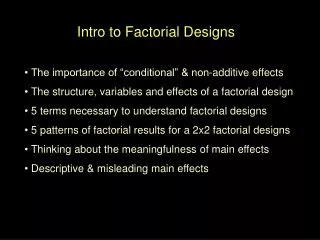
Factorial Designs: Interpretation 210 Main Effect of Exercise Significant 180 150 120 Heart Rate (beatsmin-1) Main Effect of Gender Not significant 90 60 Exercise*Gender Interaction Not significant 30 0 Exercise Resting
Factorial Designs: Interpretation 210 Main Effect of Exercise Not significant 180 150 120 Heart Rate (beatsmin-1) Main Effect of Gender Significant 90 60 Exercise*Gender Interaction Not significant 30 0 Exercise Resting
Factorial Designs: Interpretation 210 Main Effect of Exercise Not significant 180 150 120 Heart Rate (beatsmin-1) Main Effect of Gender Not Significant 90 60 Exercise*Gender Interaction Significant 30 0 Exercise Resting
Factorial Designs: Interpretation 210 180 150 ? 120 Heart Rate (beatsmin-1) 90 60 30 0 Exercise Resting
Factorial Designs: Interpretation 210 180 150 ? 120 Heart Rate (beatsmin-1) 90 60 30 0 Exercise Resting
2-way mixed model ANOVA: Partitioning Systematic Variance (resting vs exercise) = variance between means due to exercise Systematic Variance (male vs female) = variance between means due to gender Systematic Variance (Interaction) = variance between means due IV interaction Error Variance (within subjects) = uncontrolled factors plus random changes within individuals for rest vs exercise Error Variance (between subjects) = uncontrolled factors and within group differences for males vs females.
Step 1: Complete the table i.e. -square each raw score -total the raw scores for each subject (e.g. XT) -square the total score for each subject (e.g. (XT)2) -Total both columns for each group -Total all raw scores and squared scores (e.g. X & X2). Procedure for computing 2-way mixed model ANOVA
Step 2: Calculate the Grand Total correction factor GT = Procedure for computing 2-way mixed model ANOVA (X)2 N
Step 3: Compute total Sum of Squares SStotal= X2 - GT Procedure for computing 2-way mixed model ANOVA
Step 4: Compute Exercise EffectSum of Squares SSex= - GT = + - GT Procedure for computing 2-way mixed model ANOVA (Xex)2 nex (XRmale+XRfemale)2 (XEmale+XEfemale)2 nRmale+fem nEmale+fem
Step 5: Compute Gender EffectSum of Squares SSgen= - GT = + - GT Procedure for computing 2-way mixed model ANOVA (Xgen)2 ngen (XRmale+XEmale)2 (XRfem+XEfem)2 nmaleR+E nfemR+E
Step 6: Compute Interaction EffectSum of Squares SSint= - GT = + + + - (SSex+SSgen) - GT Procedure for computing 2-way mixed model ANOVA (Xex+gen)2 nex+gen (XEfem)2 (XRfem)2 (XRmale)2 (XEmale)2 nRmale nEmale nRfem nEfem
Step 7: Compute between subjectsSum of Squares SSbet= -SSgen- GT = -SSgen- GT Procedure for computing 2-way mixed model ANOVA (XS)2 nk (XT)2+(XD)2+(XH)2+(XJ)2+(XK)2+(XA)2+(XS)2+(XL)2 nk
Step 8: Compute within subjectsSum of Squares SSwit= SStotal - (SSex+SSgen+SSint+SSbet) Procedure for computing 2-way mixed model ANOVA
Step 9: Determine the d.f. for each sum of squares dftotal = (N - 1) dfex = (k - 1) dfgen = (r - 1) dfint = (k - 1)(r - 1) dfbet = r(n - 1) dfwit = r(n - 1)(k - 1) Procedure for computing 2-way mixed model ANOVA
Step 10: Estimate the Variances Procedure for computing 2-way mixed model ANOVA Systematic Variance (resting vs exercise) SSex = dfex Systematic Variance (male vs female) SSgen = dfgen Systematic Variance (Interaction) SSint = dfint Error Variance (within subjects) SSwit = dfwit Error Variance (between subjects) SSbet = dfbet
Step 11: Compute F values Procedure for computing 2-way mixed model ANOVA Systematic Variance (resting vs exercise) SSex = dfex Systematic Variance (male vs female) SSgen = dfgen Systematic Variance (Interaction) SSint = dfint Error Variance (within subjects) SSwit = dfwit Error Variance (between subjects) SSbet = dfbet
Step 12: Consult F distribution table as before Procedure for computing 2-way mixed model ANOVA Exercise Gender Interaction
2-way mixed model ANOVA: SPSS Output Systematic Varianceex SSex Calculated Fex dfex SSwit Error Variancewit dfwit
2-way mixed model ANOVA: SPSS Output GT Calculated Fgen SSgen Systematic Variancegen dfgen dfbet SSbet Error Variancebet
2-way mixed model ANOVA Systematic Variance (resting vs exercise) • The previous calculation and associated partitioning is an example of a 2-way mixed model ANOVA • i.e. exercise = repeated measures • gender = independent measures Systematic Variance (male vs female) Systematic Variance (Interaction) Error Variance (within subjects) Error Variance (between subjects)
2-way Independent Measures ANOVA Systematic Variance (resting vs exercise) • So for a fully unpaired design • e.g. males vs females • & • rest group vs exercise group Systematic Variance (male vs female) Systematic Variance (Interaction) Error Variance (within subjects) Error Variance (between subjects)
2-way Independent Measures ANOVA Systematic Variance (resting vs exercise) Systematic Variance (male vs female) Systematic Variance (Interaction) Error Variance (within subjects) Error Variance (between subjects)
2-way Repeated Measures ANOVA Systematic Variance (resting vs exercise) • …but for a fully paired design • e.g. morning vs evening • & • rest vs exercise Systematic Variance (am vs pm) Systematic Variance (Interaction) Error Variance (within subjectsexercise) Error Variance (within subjectstime) Error Variance (within subjectsinteract)
2-way Repeated Measures ANOVA Systematic Variance (resting vs exercise) Systematic Variance (am vs pm) Systematic Variance (Interaction) Error Variance (within subjectsexercise) Error Variance (within subjectstime) Error Variance (within subjectsinteract)
Summary: 2-way ANOVA • 2-way (factorial) ANOVA may be appropriate whenever there are multiple IV’s to compare • We have worked through a mixed model but you should familiarise yourself with paired/unpaired procedures • You should also ensure you are aware what these effects actually look like graphically.
Statistical Assumptions • As with other parametric tests, ANOVA is associated with a number of statistical assumptions • When these assumptions are violated we often find that an inferential test performs poorly • We therefore need to determine not only whether an assumption has been violated but also whether that violation is sufficient to produce statistical errors.
e.g. ND assumption from last year 16 17 18 19 20 Sustained Isometric Torque (seconds)
Assumptions of ANOVA • N acquired through random sampling • Data must be of at least the interval LOM (continuous) • Independence of observations • Homogeneity of variance • All data is normally distributed
“ANOVA is generally robust to violations of the normality assumption, in that even when the data are non-normal, the actual Type I error rate is usually close to the nominal (i.e., desired) value.” Maxwell & Delaney (1990) Designing Experiments & Analyzing Data: A Model Comparison Perspective, p. 109 “If the data analysis produces a statistically significant finding when no test of sphericity is conducted…you should disregard the inferential claims made by the researcher.” Huck & Cormier (1996) Reading Statistics & Research, p. 432
Group A Placebo Group B Supplement 1 Group C Supplement 2
Many texts recommend ‘Mauchley’s Test of Sphericity’ • A χ2 test which, if significant, indicates a violation to sphericity • However, this is not advisable on four counts: • 1.) • 2.) • 3.) • 4.)
Managing Violations to Sphericity • How should we analyse aspherical data? • Option 1 • Option 2 • Option 3
ANOVA is a generally robust inferential test Unpaired data are susceptible to heterogeneity of variance only if group sizes are unequal Paired data are susceptible to asphericity only if multiple comparisons are made Suggested solutions for the latter include either MANOVA or epsilon corrected df depending on sample size relative to number of levels. Summary ANOVA and Sphericity