Download

1 / 27
270 likes | 286 Vues
This analysis focuses on the refractivity of the boundary layer using CSU-CHILL radar data. It explores the algorithm description, meteorological implications, and the potential for high-resolution meteorological predictions.

E N D
The Analysis of Boundary Layer Refractivity Using the CSU-CHILL Radar David Coates
Overview • Background Information • Boundary layer refractivity • Meteorological Implications • Algorithm Description • Progress • Future Work
Refractivity • Refractivity is an optical phenomenon in which light changes its speed and orientation upon changing mediums • The relationship between speed and orientation of a ray of light in a medium is given by a medium’s index of refraction, n • The index of refraction is defined as the ratio of the speed of light to the speed of the light in a given medium
Boundary Layer (BL) Refractivity • In the atmosphere, the index of refraction depends largely on the temperature, pressure, and moisture content of the air • These variables are directly related to density, and variations in each can cause large variations in air density • Within the BL, temperature, pressure, and moisture content vary largely from location to location
BL Refractivity • Empirically, the relationship between temperature, pressure, and moisture content can be described as: p e N = 77.6 + 3.73 x 10⁵ T T2 • where p is the station pressure, T is the station temperature, and e is the vapor pressure • N, the refractivity, can be related to the index of refraction via N = (n-1)x 106
BL Refractivity • It is impossible for radar to measure any of these variables directly, so the value of refractivity must be inferred • Refraction of the electromagnetic pulses emitted from radar sites can be measured by determining the phase shift of the pulse • Radar software suites have the capability to measure the refraction undergone by backscattered radiation from distant targets
BL Refractivity • The relationship between the index of refraction of the local atmosphere and the average phase shift of a backscattered pulse is given as: R 4r ∫ φ = n[x(r), y(r), z(r), t] dr λ 0 where φ is the phase shift of the pulse, r is the distance to the target, and λ is the wavelength of the transmitted pulse
BL Refractivity • Given how small the changes in the index of refraction are, distance measurements need to be accurate to the tenth of a millimeter • This isn’t practical, so another method can be employed • Rather than scanning targets on the fly, a calibration can be made and differences in phase can be measured: R 4r ∫ φ - φref = [n(x, y, z, t1) – nref(x, y, z, t0)] dr λ 0
Meteorological Implications • Current observational networks do not have a high enough resolution to make small-scale meteorological predictions • Resolution issues on both spatial and temporal scales • Unlike ASOS, AWOS, and other meteorological observation suites, weather radar has the capability to make small-scale measurements in rapid succession
Meteorological Implications • Ideally, this method of measuring atmospheric temperature, pressure, and moisture fields at high resolution allows for meteorologists to make more accurate predictions • Specifically, in regards to convective activity, horizontal differential thermal and moisture fields can give great insight to predicted specific locations of convection initiation
Algorithm Description • In order to develop a reference phase, a calibration stage must be carried out • After calibration, test scans are analyzed by the algorithm, which calculates and smooths the refractivity field of the surrounding atmosphere • There are two modes of function: research and real-time
Archived CHILL Data Refractivity Algorithm (Research Mode) NetCDF Files csuarch2netcdf Parameter File Parameter File n_calib Reference Phase n_xtract Target Reliability Refractivity Fields
Refractivity Algorithm (Real Time) Archived CHILL Data Real-Time CHILL Data csuarch2netcdf Parameter File Parameter File NetCDF Files Target Reliability n_calib n_xtract Reference Phase Refractivity Fields
main n_calib.cpp startup get_menu_entry get_file_set build_file_list get_params add_search_path read_list confirm_do_reliability getkeyval confirm_do_calibration calib_targets find_reliable_targets read_data_foray read_data_foray
main n_xtract.cpp startup wait_rt_data get_targets free_arrays get_params read_foray_data get_file_list build_file_list get_quality read_file_list dif_phase fit_phases save_info generate_products mean_phase_slope generate_full_n_prod phase_range0 compute_test_factors write_text do_smoothing get_station mean_phase_slope write_data_foray
Algorithm Description • Separate calibrations need to be made for each season • Seasonal changes in vegetation can alter size and movement of ground targets • Season temperature swings can induce bias in the algorithm • Attention to the surrounding surface features also needs to be taken into consideration • Orographic features can results in anomalous propagation of pulses and can result in errors
Algorithm Description • Calibration produces two products to pass into the analysis program: a target reliability diagram and a reference phase plot • Special attention needs to be paid to both, as poor reliability or phase contamination can result in erroneous results
Algorithm Description Bad Target Reliability Good Target Reliability Tgt. Rel. 185900 to 182729 Tgt. Rel. 20100602
Algorithm Description Bad Reference Phase Good Reference Phase Ref. Phase 185900 to 182729 Ref. Phase 20100602
Algorithm Description • Analysis portion of the algorithm outputs two products: refractivity field imagery and netCDF files containing data arrays • Field imagery includes averaged refractivity field, scan-to-scan differential refractivity, velocity, reflectivity, and 12-hour average refractivity change • This plot can be used to determine how moisture and temperature fields change as meteorological phenomena take place
Progress • Calibration of the algorithm was achieved using a dataset from 10 December 2010 between 1941 and 2020Z • Analysis was attempted on two datasets • 13 December 2010 • 19 Jan 2011 • Output from algorithm was compared to a nearby observation station to determine validity
Progress – Refractivity Output Calculated N = 257.9
Progress – Refractivity Output Calculated N = 248.23
Progress – Refractivity Output Calculated N = 253.6
Progress – Status of Algorithm • The refractivity algorithm currently runs without error, though there are still bugs in its computational components • Possible causes: • Errant files in analysis datasets • Incorrect usage of radar constants • Poor approximations/bad object usage in algorithm language • Poor reference phase field
Future Work • In order to ensure that the algorithm outputs realistic estimations of local refractivity fields, extensive debugging is still necessary • Determine the source of the erroneous calculations and fix them