Download
1 / 75
750 likes | 1.01k Vues
Topic 3: National Income: Where it Comes From and Where it Goes (chapter 3) revised 9/21/09. Introduction. In the last lecture we defined and measured some key macroeconomic variables. Now we start building theories about what determines these key variables.

E N D
Topic 3: National Income:Where it Comes From and Where it Goes (chapter 3) revised 9/21/09
Introduction • In the last lecture we defined and measured some key macroeconomic variables. • Now we start building theories about what determines these key variables. • In the next couple lectures we will build up theories that we think hold in the long run, when prices are flexible and markets clear. • Called Classical theory or Neoclassical.
The Neoclassical model Is a general equilibrium model: • Involves multiple markets • each with own supply and demand • Price in each market adjusts to make quantity demanded equal quantity supplied.
Neoclassical model The macroeconomy involves three types of markets: • Goods (and services) Market • Factors Market or Labor market , needed to produce goods and services • Financial market Are also three types of agents in an economy: • Households • Firms • Government
Three Markets – Three agents LaborMarket hiring work FinancialMarket borrowing borrowing saving Firms Households Government production government spending investment consumption GoodsMarket
Neoclassical model Agents interact in markets, where they may be demander in one market and supplier in another 1) Goods market: Supply: firms produce the goods Demand: by households for consumption, government spending, and other firms demand them for investment
Neoclassical model 2) Labor market (factors of production) Supply: Households sell their labor services. Demand: Firms need to hire labor to produce the goods. 3) Financial market Supply: households supply private savings: income less consumption Demand: firms borrow funds for investment; government borrows funds to finance expenditures.
Neoclassical model We will develop a set of equations to charac-terize supply and demand in these markets Then use algebra to solve these equations together, and see how they interact to establish a general equilibrium. Start with production…
Three Markets – Three agents LaborMarket hiring work FinancialMarket borrowing borrowing saving Firms Households Government production government spending investment consumption GoodsMarket
Part 1: Supply in goods market: Production Supply in the goods market depends on a production function: denoted Y = F (K,L) Where K = capital: tools, machines, and structures used in production L = labor: the physical and mental efforts of workers
The production function • shows how much output (Y ) the economy can produce fromKunits of capital and Lunits of labor. • reflects the economy’s level of technology. • Generally, we will assume it exhibits constant returns to scale.
Returns to scale Initially Y1= F (K1,L1) Scale all inputs by the same multiple z: K2 = zK1 and L2 = zL1 for z>1 (If z = 1.25, then all inputs increase by 25%) What happens to output, Y2 = F (K2,L2) ? • If constant returns to scale, Y2 = zY1 • If increasing returns to scale, Y2 > zY1 • If decreasing returns to scale, Y2 < zY1
Exercise: determine returns to scale Determine whether the following production function has constant, increasing, or decreasing returns to scale:
Assumptions of the model • Technology is fixed. • The economy’s supplies of capital and labor are fixed at
Determining GDP Output is determined by the fixed factor supplies and the fixed state of technology: So we have a simple initial theory of supply in the goods market:
Three Markets – Three agents LaborMarket hiring work FinancialMarket borrowing borrowing saving Firms Households Government production government spending investment consumption GoodsMarket
Part 2: Equilibrium in the factors market • Equilibrium is where factor supply equals factor demand. • Recall: Supply of factors is fixed. • Demand for factors comes from firms.
Demand in factors market Analyze the decision of a typical firm. • It buys labor in the labor market, where price is wage, W. • It rents capital in the factors market, at rate R. • It uses labor and capital to produce the good, which it sells in the goods market, at price P.
Demand in factors market Assume the market is competitive: Each firm is small relative to the market, so its actions do not affect the market prices. It takes prices in markets as given - W,R, P.
Demand in factors market It then chooses the optimal quantity of Labor and capital to maximize its profit. How write profit: Profit = revenue -labor costs -capital costs = PY - WL - RK = P F(K,L) - WL - RK
Demand in the factors market • Increasing hiring of L will have two effects: 1) Benefit: raise output by some amount 2) Cost: raise labor costs at rate W • To see how much output rises, we need the marginal product of labor (MPL)
Marginal product of labor (MPL) An approximate definition (used in text) :The extra output the firm can produce using one additional labor (holding other inputs fixed): MPL= F(K,L +1) – F(K,L)
MPL 1 As more labor is added, MPL MPL 1 Slope of the production function equals MPL: rise over run 1 The MPL and the production function Y output MPL L labor
Diminishing marginal returns • As a factor input is increased, its marginal product falls (other things equal). • Intuition:L while holding K fixed fewer machines per worker lower productivity
MPL with calculus We can give a more precise definition of MPL: The rate at which output rises for a small amount of additional labor (holding other inputs fixed): MPL = [F(K, L +DL) – F(K, L)] / DL • where D is ‘delta’ and represents change • Earlier definition assumed that DL=1. F(K, L +1) – F(K, L) • We can consider smaller change in labor.
MPL as a derivative As we take the limit for small change in L: Which is the definition of the (partial) derivative of the production function with respect to L, treating K as a constant. This shows the slope of the production function at any particular point, which is what we want.
The MPL and the production function Y output MPL is slope of the production function (rise over run) F(K, L +DL) – F(K, L)) L labor
L: 1 4 9 F(L): 3 6 9 fL: 1.5 0.75 0.5 Derivative as marginal product Y 9 6 3 L 4 9 1
Return to firm problem: hiring L Firm chooses L to maximize its profit. How will increasing L change profit? D profit = D revenue - D cost = P * MPL - W If this is: > 0 should hire more < 0 should hire less = 0 hiring right amount
Firm problem continued So the firm’s demand for labor is determined by the condition: P *MPL = W Hires more and more L, until MPL falls enough to satisfy the condition. Also may be written: MPL = W/P, where W/P is the ‘real wage’
Real wage Think about units: • W = $/hour • P = $/good • W/P= ($/hour) / ($/good) = goods/hour The amount of purchasing power, measured in units of goods, that firms pay per unit of work
Example: deriving labor demand • Suppose a production function for all firms in the economy:
Three Markets – Three agents LaborMarket hiring work FinancialMarket borrowing borrowing saving Firms Households Government production government spending investment consumption GoodsMarket
Units of output Real wage MPL, Labor demand Units of labor, L MPL and the demand for labor Each firm hires labor up to the point where MPL = W/P
Determining the rental rate We have just seen that MPL= W/P The same logic shows that MPK= R/P: • diminishing returns to capital: MPK as K • The MPKcurve is the firm’s demand curve for renting capital. • Firms maximize profits by choosing Ksuch that MPK = R/P.
How income is distributed: We found that if markets are competitive, then factors of production will be paid their marginal contribution to the production process. total labor income = total capital income =
nationalincome capitalincome laborincome Euler’s theorem: Under our assumptions (constant returns to scale, profit maximization, and competitive markets)… total output is divided between the payments to capital and labor, depending on their marginal productivities, with no extra profit left over.
Mathematical example Consider a production function with Cobb-Douglas form: Y = AKL1- where A is a constant, representing technology Show this has constant returns to scale: multiply factors by Z: F(ZK,ZY) = A (ZK) (ZL)1- = A Z K Z1- L1- = A Z Z1- K L1- = Z x A KL1- = Z x F(K,L)
Mathematical example continued • Compute marginal products: MPL = (1-) A KL- MPK = A K-1L1- • Compute total factor payments: MPL x L + MPK x K = (1-) A KL-x L + A K-1L1-x K = (1-) A KL1- + A KL1- = A KL1- =Y So total factor payments equals total production.
Three Markets – Three agents LaborMarket hiring work FinancialMarket borrowing borrowing saving Firms Households Government production government spending investment consumption GoodsMarket
Outline of model A closed economy, market-clearing model Goods market: • Supply side: production • Demand side: C, I, and G Factors market • Supply side • Demand side Loanable funds market • Supply side: saving • Demand side: borrowing DONE Next DONE DONE
Demand for goods & services Components of aggregate demand: C = consumer demand for g & s I = demand for investment goods G = government demand for g & s (closed economy: no NX )
Consumption, C • def: disposable income is total income minus total taxes: Y – T • Consumption function: C = C (Y – T ) Shows that (Y – T ) C • def: The marginal propensity to consume (MPC) is the increase in C caused by an increase in disposable income. • So MPC = derivative of the consumption function with respect to disposable income. • MPC must be between 0 and 1.
C C(Y –T ) The slope of the consumption function is the MPC. rise run Y – T The consumption function
Consumption function cont. Suppose consumption function: C=10 + 0.75Y MPC = 0.75 For extra dollar of income, spend 0.75 dollars consumption Marginal propensity to save = 1-MPC
Investment, I • The investment function is I = I (r ), where rdenotes the real interest rate,the nominal interest rate corrected for inflation. • The real interest rate is the cost of borrowing the opportunity cost of using one’s own funds to finance investment spending. So, r I
r Spending on investment goods is a downward-sloping function of the real interest rate I(r) I The investment function


![[16 th Ed.] National Income Accounting](https://cdn2.slideserve.com/4427362/16-th-ed-national-income-accounting-dt.jpg)


![[16 th Ed.] National Income Accounting](https://cdn3.slideserve.com/5747022/16-th-ed-national-income-accounting-dt.jpg)