Download
1 / 60
600 likes | 622 Vues
Learn about memory hierarchy levels, data transfer between levels, cache basics, hit rate, miss penalty, and why memory hierarchies work. Discover the principles behind memory organization and tuning for optimal performance.

E N D
Memory HierarchiesChapter 7 N. Guydosh 4/18/04
The Basics • Fake out the program (application) into thinking it has a massive high speed memory - limited only by the address space. • The appearance of a massive high speed memory system is an illusion - but the performance enhancement is real. • Will consider three levels of memory media: • Cache • Main Memory • Disk • Principle of locality(pp. 540-541)Programs access only a very small part of the address space at any instant of time • Temporal localityIf an item is referenced, it will probably be referenced again soon. • Spatial localityIf an item is referenced, items whose addresses are close by will tend to be referenced soon
Memory Hierarchy • Organize memory into “levels” according to cost speed factors: • The higher the level the faster, smaller, and more expensive (per bit) the memory is • The lower the level the slower, larger, and cheaper (per bit) the memory becomes • The highest level is directly accessed by the microprocessor. ... The cache • The levels to be considered areSRAM ... Super fast memory - expensive DRAM ... Ordinary ram memory - minimum speed - cheapDISK (DASD) ... Very slow, very cheap
Memory Hierarchy Levels Cache Main memory Disk Fig. 7.1
Data Transfer Between Levels • Block • The minimum unit of data that can be present or not present in a two level memory (cache system). It can be as small as a word or may be multiple words. • This is the basic unit of data transfer between the cache and “main” memory • At lower levels of memory, blocks are also known as “pages”:
Data Transfer Between Levels blocks Fig. 7.2
The Basic Idea • The data needed by the processor is loaded into the cache on demand • The data needed by the processor is loaded into the cache on demand • If the data is present in the cache, the processor used it directly. This is called a hit • Hit rate or ratio: • The fraction (or percent) of the time the data is found at the high level of memory without incurring a miss. • Miss rate or ratio: • 1 - hit rate (or 100 - hit rate in percent)
The Basic Idea (cont.) • Hit TimeThe time it takes to access an upper level of memory of a memory hierarch (cache for two level) • Miss penaltyThe time it takes to replace a block in an upper level of a hierarchy with a corresponding block from a lower level • A miss in a cache is serviced by hardware • A miss at a level below the cache (ex: main memory) is serviced in software by the operating system (must do I/O at disk level).
Why the Idea Works • Fundamental phenomenon or properties which make this scheme work • Hit ratios must be and are generally very high • High hit ratios are a result of the locality principle described above • Success is statistical and could never be deterministically guaranteed. A good (or bad?) Programmer could always write a program which would kill a memory hierarchy ... cause thrashing • Memory hierarchies must be tuned via level sized, block (page) sized to get optimal performances
The Basics of Caches • Simplest type: single word block • On start up the cache is empty, and as references are made, it fills up via block misses and transfers from ram • Once it “fills” locality principle takes over a there are very few misses. • Question: • Where are the blocks put in the cache and how are they found and related to main memory blocks? • There must be a mapping scheme between cache and main memory
The Basics of Caches • Direct mapping – assuming addresses are “block numbers”* • A word from memory can map into one and only one place in the cache. • The cache location is directly derived from the main memory address. • Direct mapping rule:Cache address of a block (block number) is the main memory block number “address” modulo the cache size in units of blocks • For example: if the main memory block number is 21decimal and the cache size was 8 blocks, then cache address is 21 mod 8 = 5 decimal. • If we keep the size of the cache (in blocks) a power of 2, then the cache address is directly given by the log2 (cache size in blocks) low order bits. Ex: 21(base 10) = 010101(base 2). Log28 = 3. Three low order bits are 101 = 5 decimal. • Note that Memory cache mapping is many to one (see P. 546, fig 7.5) • Preview – If this is direct mapping, then there must be a non-direct mapping … set associative … more that one place to put a block … See later.* a block number is a byte address which has the low order bits designating the word within a block, and the byte within a word stripped off. If an block were a byte, then these addresses would be “complete”.
Memory Cache MappingSpecial Case: One Word Per Block“Piano Keys” Every block (= word) in memory maps into a unique location in cache. Two low order bits for byte within a word stripped off. Fig. 7.5
Memory Cache Mapping (cont.) • Questions: • Because each cache location can contain the contents of a number of different memory locations, how do we know whether the data in the cache corresponds to a requested word ie., the block containing this word? • How do we know if a requested word is in the cache or not? • The answer is in the contents of a cache entry – blowing in the wind: • 32 bit data field - the desired raw data • Tag field: high order address after “modulo” low order cache bits stripped out – this identifies the entry with a unique memory block. • A one bit valid field (validity bit).The valid bit is turned on if a block has been moved into the cache on demand If the valid bit is, on the tag and data field are valid
How a Block is Found • The low order address bits of the block number (log cache size in blocks) from the main memory address is the index into the cache. • If the valid bit is on, the tag is compared with the corresponding field in the main memory address. • If it compares we have a hit • If it does not compare, or if the valid bit is off, we have a miss and the hardware copies the desired block from main memory to this location in cache • Whatever was at this cache location gets overlaid.
How a Block is Found One word (4 bytes) per block Byte offset within a word: bits 0,1 block (frame) number within cache: 2, …, 11 tag: 12, 13, …, 31 block number in logical space – compare with Page Table 4 bytes Cache by definition is size 210 Contrast to main memory in VM Scheme where mem size is arbitrary Fig. 7.7 Similar to DEC example Fig 7.8 Data is 32 bits Entry has 32+20+1 = 53 bits Emphasis is more on temporal rather than spatial locality
Handling a Cache Miss • Instruction miss – p. 551 • Access main memory at address PC-4 for the desired instruction block. (Read). • Write the memory data in the proper cache location (low order bits) and the upper bits in the tag field, then turn on the valid bit • Restart the instruction execution from the beginning, it will now re-fetch and find it in the cache. • A cache stall occurs by stalling the entire machine (rather than only certain instructions as in a pipeline stall.)
Handling a Page Fault • Read data miss • Similar to instruction miss - simply stall processor until cache is updated - simply retain ALU address output for processing the miss (where to move mem data in cache). • Write miss (see pp. 553-554): • If we simply write to data cache without updating main memory, then cache and memory would be inconsistent • Simple solution is to use write-through:index to cache with low order bits • Write the data and tag portion into the block & set valid, then write data word to main memory with entire address.Contrast this later to the case of more that one word per block. • This method impacts performance - an alternate approach is ==>
Handling a Page Fault (cont.) • Write buffer technique (p. 554): • Write data into cache and buffer at the same time (buffer is fast) ... processor continue execution – sort of a “lazy evaluation” . • While the processor proceeds, the buffer data is copied to memory • When write to main memory completes, the write buffer entry is freed up • If the write buffer is full when a write is encountered, the processor must stall until a buffer position frees up. • Problem: even though the writes are generated at a rate less than the rate of “absorption” by main memory (average), “bursts “ of writes can stall the processor ... only remedy is to increase buffer size. • Buffer is generally small (=< 10 words • A preview of other problems associated with caches: • In a multiprocessing scheme where each processor may have its own cache and there is a common main memory • Now we have a “cache coherency problem • Not only must we keep the caches in steep with main memory, but we must keep them in step with each other – more later.
Taking advantage of Spatial locality • Up to now there was essentially no spatial locality • Block size was too small – the unit of memory transfer to the bus is a word • The block size was one word • A block consist of multiple contiguous words from main memory • Need a cache block of size greater than one word for spatial locality • Load the desired word and its local “companions” into cache • A miss always brings in an entire block • Assume the number of words per block is a power of 2
Taking advantage of Spatial locality • Mapping an address to a multiword cache block • Example:block size = 16 bytes ==> low 4 bits is byte offset into a block ==> low 2 bits is byte offset into a word ==> bits 2 and 3 are word offset into block cache size = 64 blocks thus low 6 bits is the block number in cache.What does byte address of 1202 (decimal) = 0x4B2 map to? • Block given by (block address) mod (number of cache blocks)where block address(actually block number in “logical space”) = (byte address) / (# bytes per block) = floor(1202/16) = 75d = 0x4B … drop low 4 bit offset in blockcache block number = 75 mod 64 = 0x4B mod 64 = 11decimal = 001011b = low 6 bits of block number • Summary:1202d = 0x00004B2 = |0000 0000 0000 0000 0000 01001011| 0010 | block numbercache location | blk offsetRemember: block_address = block_number | block_offset … book is a bit sloppy. Also 001011 (in red) field is cache locationAlso: #bits in index = log2(#sets in cache) = log2((size of cache)/(size of set)) = log2(64blocks/1 block/set) = log264 = 6. … see later
64K Cache Using a 16 Byte Block 16 byte blocks directly mapping or 4 word blocks directly mapped … preview 1 way associative 64 KB = 16K words = 4K blocks = 12 bit index in cache Tag associated with block not the word 12 low bits Pick off word in a block Still direct mapping! See set associative later Fig. 7.10 Fig. 7.10
Taking advantage of Spatial locality Miss Handling • Read miss handling • Processed the same way as a single wordblock read miss • A read miss always brings back the entire block
Taking advantage of Spatial locality Miss Handling (cont.) • Write miss handling • Can’t simply write the data and corresponding tag because block contains more than a single word. • When we had one word per block, we simply wrote the data and tag into the block & set valid, then write data word to main memory. • Must now first bring in the correct block from memory if the tagmismatches, and then update the block using write-through or buffering. If we simple wrote the tag and word, we could possible be “updating” the wrong block (intermixing two blocks) … multiple blocks could map to the same cache location.See bottom page 557.
Tuning Performance With Block Size • Very small blocks may lose spatial locality (ex. 1 word/block) • Very large blocks may reduce performance if the cache is relatively small - competition for space • Spatial locality occurs over a limited address range - large blocks may bring in data which will never get referenced – “dead wood”. • Miss rate may increase for very large blocks
Tuning Performance With Block Size (cont.) Fig. 7.12 Cache size Cover cache performance later
Performance Considerations • Assume that a cache hit gives “normal” performance, that is, this is our base line for no performance degradation – peak performance. • We get performance degradation when a cache miss occurs. • Recall that a “cache stall” occurs by stalling the entire machine (rather than only certain instructions as in a pipeline stall.) • Memory stall cycles are “dead” cycles elapsing during a cache stall. This consists of: • Memory-stall clock cycles = read-stall cycles + write-stall cycles.For example on a per program basis.Where: • Read-stall cycles = (reads/program) x (read miss rate) x (read miss penalty)where read miss penalty is in cycles, and may be given by some formula involving say block size. • Write-stall cycles = (writes/program) x (write miss rate) x (write miss penalty) + write buffer stallswhere write buffer stalls accounts for the case where a buffer is used to update main memory when a cache write occurs. If write buffer stalls are a significant part of the equation, it probably means this is a bad design! We shall assume a good design where the buffer is deep enough for this to be an insignificant term
Performance Considerations (cont.) • Assuming that the read and write miss penalty are the same, and that we can neglect write buffer stalls, we can write a more general formula:. • Memory-stall clock cycles = [(memory accesses)/program ] x (miss rate) x (cache miss penalty) • For example in homework problem 7.27, the cache miss penalty we given by the formula: 6 + (block size in words) number of cycles. • An example (page 565) ==>
Performance Considerations (cont.) • Assuming an instruction cache miss rate for gcc of 2% and a data cache miss rate of 4%. If a machine has a CPI of 2 without any memory stalls (ie., ideal case of no cache misses), and the miss penalty is 40 cycles for all misses, determine how much faster a machine would run with a perfect cache that never misses. Use instruction frequencies from page 311 of text. • For instruction count I:instruction miss cycles = I x 2%x 40 = 0.80I • Data miss cycles = I x 36% x 4% x 40 = 0.56Iwhere the frequency of instructions doing memory references is 35% from page 311 • Total memory stall cycles = 0.80I + 0.56I = 1.36I > 1 cycle of memory stall per instruction. • The CPI with stalls = 2 + 1.36 = 3.36 • Thus: (CPU time with stalls)/(CPU time for perfect cache) =[IxCPIstall x (clock cycle time)]/[I x CPIperfect x (clock cycle time)] = CPIstall / CPIperfect = 3.36/2 = 1.68 … ideal case is 68% better.
Performance Considerations (cont.)$ • Effects of cache/memory interface options on performance • Cache interacts with memory for cache misses • Goal:minimize block transfer time (maximize bandwidth)minimize cost • Must deal with tradeoffs • Cache and memory communicate over a bus – generally not the main bus • Assume memory is implemented in DRAM and cache in SRAM • Miss penalty (MP) is the time (in clock cycles) it takes to transfer between memory and cache • Bandwidth is the bytes/second to transfer a block • Example:Assume: 1 clock cycle to send address to memory (just need initial address) 15 clock cycles for each DRAM access initiated … effective access time 1 clock cycle to send a word to cache • Bandwidth = (words/block)/(miss penalty) • See fig. 7.13 for three cases ==>
Bandwidth Example$ ------------4 words -------- MP = 1+1x15 +4x1 = 20 cycles BW = (4x4)/20 = 0.8… read 4 words in parallel and Deliver to cache one word at a time 1 word --- MP = 1+1x15 +1x1 = 17 cycles BW = (4x4)/17 = 0.94 … read 4 words in parallel and Deliver to cache 4 words at a time Miss penalty (MP) = 1+4x15 +4x1 = 65 cycles Bandwidth = BW = (4x4)/65 = 0.25 … read 1 word from memory and deliver to cache one word at a time Fig. 7.13
Now Comes Amdahls Law! • Summary:CPIstall / CPIperfect = 3.36/2 = 1.68 … ideal case is 68% better • Lets speed up the processor • The amount of time spent on memory stalls will take up an increasing fraction of the execution time. • Example: speed up the CPU by reducing CPI from 2 to 1 without changing he clock rate. • The CPI with cache misses is now 1 + 1.36 = 2.26perfect cache is now 2.36/1 times faster instead of 3.36 faster • Amount of execution time spent on memory stalls would have risen: from: 1.36/3.36 = 41% (slow CPU) to: 1.36/2.36 = 58% (fast CPU) ! • Similar situation for increasing clock rate without changing the memory system.
The Bottom Line • Relative cache penalties increase as the machine becomes faster – thus if a machine improves both clock rate and CPI, it suffers a double hit. • The lower the CPI, the more pronounced the impact of stall cycles. • If main memory of two machines have the same absolute accesses times, the higher CPU clock rate leads to a larger miss penalty. • Bottom line put the improvement where it is needed: improve memory system not CPU.
More Flexible Placement of Blocks“Set Associative” • Up to now we used direct mapping for block placement in the cache • Only one place to put a block in cache. • Finding a block is easy and fast • Simple directly address it with low order block number bits. • The other extreme is “fully associative” • A block could be placed anywhere in the cache. • Finding a block is now more complicated: must “search” the cache looking for a match on the tag. • In order to keep the performance high, we do the search in hardware (see later) at a cost tradeoff • Let us look at schemes between these two extremes.
Set Associative Block Placement • There is now a fixed number of locations (at least two) where a block can be placed • For n locations it is called an n-way associative cache • An n-way associative cache consists of a number of sets, ech having n blocks • Each block in memory maps to a unique set in the cache using the “index field” (low “mod” bits). • Recall that in a direct mapped cache, the position of a memory block was given by: (block number) mod (number of cache blocks) … low order block # bits • Note that the number of cache blocks in this case is same as the number of sets … one block per set. • In general use set-associative cache: the set number containing the desired memory block is given by:(block number) mod (number of sets in the cache) .Again this is low order block # bits • See diagram ==>
Set Associative Block Placement (cont.) Direct mapped Set associative Fully associative 8 sets – 8 blocks 4 sets – 8 blocks 1 set – 8 blocks Set 0 (one set) Block = set 12 mod 8 = 4 Set 12 mod 4 = 0 Fig. 7.15 One tag per set Example above uses cache block number of 12 dec = 0xC= 1100 bin Note: 0xC results when block offset bits stripped off.
Definition: the (logical) “size” or “capacity” of a cache usually means the amount of “real” or “user”data it can hold. The physical size is larger to account for tags and status bits (such as valid bits) also stored there. Set Associative Block Placement (cont.)%%% Set = Definitions:Associatively = #blocks/set A block is one or more words The “Tag” is associated with a block within a set. Fig. 7.16
Set Associative Mapping • For direct mapped, the location of a memory block (one or more words) given by:index =(Block number) mod (number of cache blocks) • For a general set associative cache, the set containing a memory block is given by:index =(Block number) mod (number of sets in the cache) • This is consistent with the direct mapped definition, since for direct mapped, there was one block per set. • Each block in memory maps to a unique set in the cache given by the index field. • The placement of a block within a set is not unique – it depends on a replacement algorithm (example LRU). • Must logically search a set to find a particular block identified by its tag. • The tag is the high order remaining bits after the index and offset into the block is stripped off. • In the case of fully associative (only one set), there is no index because there is only one place to “index” into – ie., the entire cache. • The number of bits in the index field is determined by the size of the cache (in units of sets). The size of a set is the block size x the associatively of the set.
Set Associative Mapping (cont.) |<-------block number------------->| index =(block number) mod (number of sets in the cache) block size = 2(number of bits in block offset) bytes number of bits in index = Log2(number of sets in cache) number of bits in index is directly a function of the size of the cache* and the associativity of the sets. number of bits in index = Log2[ (size of cache)/(size of set) ] = Log2[ (size of cache)/(associativity of set**)(size of block) ] … consistent units must be used in calculations (bytes, words, etc.) * Size of cache mean the amount of “real” data it holds. It does not account for validity and tags stored. **Assumes associativity of set is defined as number of blocks in a set.
Set Associative Block Placement (cont.)Example 4 – way associative Block# =tag | index Block size = 1 word = 4 bytes block offset(2 bits) tag index #bits in index = = log2(#sets in cache) = log2[(cache size)/set size)] =log2[1024/4]= log2(256)=8 Cache size = #sets x size of set = 256 x 4 words = 1024 words =4Kbytes Fig. 7.19
Set Associative Mapping – an Example pp. 571-572 Cache size = 4 words = 4 blocks Sequence of block numbers: 0, 8, 0, 6, 8 CASE 1: direct mapping: one block per setthus # sets in cache = 4 # index bits = log2(#sets in cache) = log2[(cache size)/(set size)] = = log2[4/1] = 2 bits in the index The tag must have 32 – 2 bits in index – 2 bits in block offset = 28 bits |<-------block number---------------------------->|blk offset 31 … 4 3 2 1 0 Tag: bits 4 … 31Index: bits 2,3 Block offset: bits 0,1block # = 0 ==> set index = (0 mod 4) = 0 block# = 6 ==> set index = (6 mod 4) = 2 block# = 8 ==> set index = (8 mod 4) = 0 Total of 5 misses – see text.
Set Associative Mapping – an Example pp. 571-572 Cache size = 4 words = 4 blocks Sequence of block numbers: 0, 8, 0, 6, 8 CASE 2: 2 – way associative mapping: two blocks per setthus # sets in cache = 4 blocks/(2 blocks/set) = two sets in the cache # bits in index = log2(#sets in cache) = log22 = 1 bit in the index The tag must have 32 – 1 bits in index – 2 bits in block offset = 29 bits |<-------block number---------------------------->|blk offset 31 … 3 2 1 0 Tag: bits 3 … 31 Index: bit 2 Block offset: bits 0,1block # = 0 ==> set index = (0 mod 2) = 0 block# = 6 ==> set index = (6 mod 2) = 0 block# = 8 ==> set index = (8 mod 2) = 0 Total of 4 misses – see text. – use LRU for replacement
Set Associative Mapping – an Example pp. 571-572 Cache size = 4 words = 4 blocks Sequence of block numbers: 0, 8, 0, 6, 8 CASE 3: fully associative mapping: 1 set, 4 blocks per setthus # sets in cache = 4 blocks/(4 blocks/set) = one set in the cache # bits in index = log2(#sets in cache) = log21 = 0 bits in the index The tag must have 32 – 0 bits in index – 2 bits in block offset = 30 bits |<-------block number--------------------------->|blk offset 31 … 2 1 0 Tag: bits 2 … 31 Index: none Block offset: bits 0,1block # = 0 ==> set index = (0 mod 1) = 0 block# = 6 ==> set index = (6 mod 1) = 0 block# = 8 ==> set index = (8 mod 1) = 0 Total of 3 misses – see text. – use LRU for replacement
Virtual Memory • An extension of the concepts used for cache design (or maybe vise-versa?) • Key differences: • The cache is now main memory • The backing store is now a hard drive • The size of logical space is now orders of magnitude larger and in a cache scheme • The hardware “search” on the tag used in locating a block in a cache, is no longer feasible in a VM scheme • A fully associative scheme is used in order to get the highest hit ratio • No restrictions on where the block (page) goes • Dragging along a tag is prohibitive in space usage • Searching for a tag is also not practical – too many of them • Thus software is used and addresses are mapped using a page table • Sometimes the PT is “cached” using a TLB which works like a cache
Virtual Memory Mapping Virtual page Fig. 7.23
Virtual Memory Mapping Virtual address Fig. 7.21
Virtual Memory Mapping Fig. 7.22
Page Faults • Page Faults • If the page referenced by the virtual address is not in memory we have a page fault. • A page fault is determined by checking the valid bit in the page table entry indexed by the virtual page number. • If valid bit is off we have a page fault • Response to a page fault • An exception is raised, and the OS takes over to fetch the desired page from memory. • Must keep track of disk address to do this • Disk addresses typically kept in page table – but there are other schemes also (p. 586) • If memory has an unused page frame, then load the new page there. • If memory is “full” choose an existing valid memory page to be replaced – if this page is modified, disk must be updated.
Page Faults (cont.) • How to we locate the page to be brought in from the disk? • Need a data structure similar to the page table to keep track of map virtual page number to disk. • One way is to keep disk addresses in the page table along with real page numbers – other schemes may be used also. • Used for reading from as well as writing to disk. • Where do you put the page from disk if memory is “full”? • Replace some existing page in memory which is least likely to be needed in the future. • Least Recently Used (LRU) algorithm commonly used. • LRU in its exact form is costly to implement. • LRU status updates must be made on each reference. • At least from a logical point of view, must manage an LRU stack • A number of LRU approximations possible which are more realistic to implement – example: use a reference bit(s) and only replacing pages whose reference bits are off.
Writes to the Memory System • What about writes to cache? • Must keep main memory in step with cache • Use “write through” or write buffer to memory for cache writes • Write buffer hides the latency of writing to memory. • Main memory updated at the time of write. • What about writes to memory? • Must keep disk backing store in step with memory • Disk access is too slow to use write through. • Use “lazy evaluation” and do updates only on a replacement. • Write back only when page is to be replaced or when process owning the page table ends – minimizes disk access. • Keep track of modified pages with a “dirty bit” in page table.
Virtual Memory Mapping (Cont.)Houston – We have a problem! • We have both a space and time problem • Space would be bad enough but time also! • Page tables can be huge. • If the address is 32 bits and the page size is 2K, then there are 221 2 Million entries at, say, 4 bytes per entry = 8 Megabytes! • To make matters worse, each process has a page table. • Memory access time is doubled • Even for a page hit, we must first access access the page table stored in memory, and then get the desired data, • Two memory accesses to get the desired data in the most ideal situation (a page hit).