Download
1 / 59
590 likes | 754 Vues
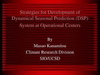
Strategies for Development of Dynamical Seasonal Prediction (DSP) System at Operational Centers. By Masao Kanamitsu Climate Research Division SIO/UCSD. Preface. Operational vs. Research Statistical vs. Dynamical. Operational vs. Research. Operational Produce useful results now!

E N D
Strategies for Development of Dynamical Seasonal Prediction (DSP) System at Operational Centers By Masao Kanamitsu Climate Research Division SIO/UCSD
Preface Operational vs. Research Statistical vs. Dynamical
Operational vs. Research • Operational • Produce useful results now! • whatever the method is. • Research • Great future potential • Does not produce useful results now • Take time (and money)
Operational vs. Research • Requires balanced thinking. Do not go too much towards one direction. • Think science • Promote understanding between managers and developers
Statistical/Empirical vs. Dynamical • Statistical • Relatively easy and fast • Produces results now • Skill statistically assured • Not much future (statistical limitation) • Dynamical • Difficult • May take time to produce useful results • Skill not assured • Great potential for future
Current Status of Statistical/Empirical Methods • Statistical method based on EOF is now well established. Currently, most reliable method. • CCA* • Composites* • Trend (persistence)* • Extrapolation of phase, amplitude* • Identification of “modes”. *) applies to forecast over Taiwan
Current DSP status (1) • Current products are NOT as useful as we hope for operational seasonal forecasts. • Still the method is not matured • It is an investment for future. • 5-years? 10-years? • Need to be up-to-date to be competitive with other centers
Current DSP status (2) • May be useful in particular situations • This is still not demonstrated • Progress in modeling and research may make the DSP as useful tool in a short time.
Statistical: ANALOG NEURAL CCA SSA/MEM (LIM) Dynamical (simple): OXFORD LDEO SCR/MPI BMRC Dynamical (2-tier) NCEP Dynamical (1-tier?) COLA After Landsea amd Knaff (2000) Skill measured against persistency/climatology
Basic approaches to seasonal forecasting • Phenomenological approach • Atmospheric “modes” approach * • Specific external forcing approach * • Pure empirical approach • Dynamical Modeling *
Phenomenological consideration(what phenomena to predict) • Summer monsoon (Meiyu) • Winter monsoon (cold surges) • Typhoon • Subtropical highs Be aware that our interest is the prediction of “anomaly”
Application to Prediction- phenomenological - • Normally does not help making predictions • Help targeting what to predict • Physical understanding of the mechanism helps what to look and how to model.
Atmospheric modes Decompose/extract typical signal from complex atmospheric patterns. Convenient tool*
Consideration from “Modes” • Madden Julian Oscillation (MJO)* • Pacific North America (PNA) pattern* • North Atlantic Oscillation (NAO) • Arctic Oscillation (AO), Annular mode.* • Pacific Decadal Oscillation (PDO)* • Pacific Japan (PJ) pattern* • Many other patterns*
Examples of various “modes” NAO* PNA*
Examples of various modes AO Thompson and Wallace (2000)
Examples of various modes PJ Nitta (1987)
Examples of various modes MJO Waliser et al. (2000)
Application to Prediction- Modes - • Use as input/output for statistical method • Composite maps based on modes • Extrapolate phase and amplitude • Physical understanding of the mechanism helps what to look and how to model
External Forcing (1) • Sea Surface Temperature • This is what started DSP • Use as input for statistical method (CCA) • Direct impact in tropics* • Nordeste, Indonesia precipitation,Taiwan(??) • Remote response • ENSO =>PNA • Western Pacific (Phillipines) => PJ • Indian Ocean dipole
ENSO Impacts Halpert and Ropelewski (1992)
External Forcing (2) • Soil moisture • Normally local • Summer season • Delayed SST impact via soil moisture • Snow • Similar to Soil moisture • Delayed effect • Sea-ice • Vegetation, urbanization • CO2, ozone and other greenhouse gasses
Application to prediction - External forcing - • Use as input in statistical methods • Composite • Key factor for dynamical seasonal forecasts • How to predict external forcing?
Pure empirical approach • Analog method • Pattern recognition • Constructed analog • Using the behaviors of animals, plants and other natural phenomena. Lacks scientific basis Not recommended !!!
Application to prediction - Dynamical - • Based on physical principles • Most promising • Should be able to predict rare events (in principle, even events not occurred in history)
DSP Approach • Identify sources of predictability • Dynamical consistency • Signal to noise • Systematic error
Source of seasonal predictability • SST • Soil wetness • Snow • Sea ice • CO2, ozone and other trace gasses for trend • Initial conditions, particularly ocean, land Need for incorporating as many predictability sources as possible into the system. Discourages simplification. Need for coupled modeling
Dynamical Consistency • Two-tier (one-way coupling) • One-tier (two-way coupling) should be one-tier MJO example Extra tropical sst example
Signal and noise (1) • In seasonal forecasts, transient disturbances with the frequency less than about 30 days are considered to be “noise”. • The targets of prediction for short-range and medium-range are noise in seasonal forecast. • Lorenz’s chaos theory • Infinitesimally small difference in initial condition results in very large differences after 2 weeks. • There is no way to avoid this “noise”. • You need to consider that the highs and lows in the middle latitudes in real atmosphere is also a “noise”. We describe nature as “One of many realizations”.
Example of signal to noise ratio Sugi et al (1997)
Signal and noise (2) • If there is no external forcing, atmospheric mean state is not predictable. • Signal is the pattern that shows up on all the predictions regardless of the “noise”.
Signal and noise (3) • Why predict “noise” • Middle latitude disturbances are essential component of general circulation. Transport heat and momentum. • Low frequency model and difficulties of parameterizing time mean effect of transient disturbances. • Prediction of individual disturbances need not be accurate, but time mean property of the transient disturbances need to be accurate. • This is in good analogy to cumulus parameterization.
Signal and noise (4) • Thus, ensemble forecasting is an essential part of the seasonal prediction. • One integration provides only on “realization” • All the seasonal forecasts need to be probabilistic.
Signal and Noise (5) • Theory on Seasonal Ensemble forecasting • Sardeshumukh (2000) • Number of ensemble members required • Simple mean (order of 20-40) • Second moment (order of a few hundred) • Skewness (even more)
Systematic Error • Average of many forecasts minus corresponding observation. • Model mean error • Model climatology • Fairly large amplitude • Cannot use the model forecast “as is” • Systematic error correction • Assuming there is no interaction between systematic error and model dynamics. This is a big assumption! • Built-in statistical correction to dynamical model
Example of the importance of systematic error correction Kanamitsu et al (2002)
1st recommendation • Use statistical method as one of the leading methods for operational forecast. • CCA • Composite • Extrapolation of “modes” • Persistency (or trend) • Other statistical method with some physical basis. • Do not go into “pure empirical” without any physical basis => my personal opinion.